Spagna 2010

P1.- Zancos saltadores

El inspector Gadget, personaje de una serie de cómic, utiliza unos muelles pegados a sus zapatos para realizar saltos espectaculares. Algunos deportistas atrevidos intentan emularlo, utilizando unos zancos desarrollados por la industria aeroespacial que les permiten dar saltos de casi 2 m o hacer “footing” a más de 40 km/h (figura 1).

El estudio detallado de la mecánica de estos saltos es complicado. Para simplificarlo, vamos a adoptar un modelo sencillo constituido por un bloque de masa $m$ sujeto a la parte superior de un muelle ideal sin masa, de longitud natural $L_0$ y constante elástica $k$.

Si dejamos caer el sistema, partiendo $m$ de una altura inicial $y_{\mathrm{ini}}$ (figura 2a), caerá verticalmente, chocará con el suelo y rebotará hacia arriba. Durante el descenso, $m$ pasa sucesivamente por tres posiciones singulares:

• El extremo inferior del muelle alcanza el suelo (figura 2b).
• El bloque pasa por una altura, $y_{\mathrm{eq}}$, en la que la fuerza neta que actúa sobre él es nula (figura 2c). Esta sería la altura del bloque en equilibrio si el sistema se apoyase suavemente sobre el suelo.
• El bloque se detiene momentáneamente a una altura mínima, $y_{\min }$, antes de empezar a subir (figura 2d).

Supón que se conocen $L_0$, $y_{\mathrm{ini}}$ e $y_{\min }$, además de la aceleración de la gravedad, $g$. Contesta las siguientes preguntas, expresando tus resultados en función de los datos anteriores:

a) Determina la relación $k/m$ entre la constante del muelle y la masa del bloque.

b) Determina la altura de equilibrio, $y_{\mathrm{eq}}$.

c) Describe la aceleración de $m$ en los siguientes intervalos:

• Desde $y=y_{\mathrm{ini}}$ hasta $y=L_0$.
• Desde $y=L_0$ hasta $y=y_{\min }$.

d) En la caída, ¿a qué altura $y_1$ es máxima la aceleración del bloque? ¿Cuál es su valor, $a_{\max }$?

Para las dos siguientes preguntas, toma como datos numéricos: $L_0=80\text{ cm};y_{\mathrm{ini}}=2,0\text{ m};y_{\min }=20\text{ cm};g=9,8{\text{ m/s}}^2.$

e) Calcula los valores de $k/m$, $y_{\mathrm{eq}}$ y $a_{\max }$.

f) Haz una representación gráfica de $a/g$ en función de $y$, para $y_{\min }\le y\le y_{\mathrm{ini}}$.

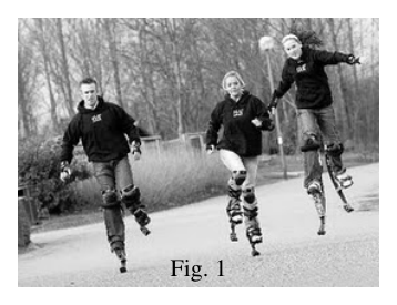Foto de zancos saltadores (Fig. 1)

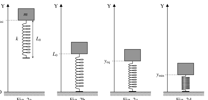Diagrama posiciones caída muelle-masa (Fig. 2)

Topic: Oscillations & Waves, Newtonian Mechanics, Conservation of Energy Metodi: Hooke’s Law, Free-Body Diagram, Conservation of Energy, Kinematic Equations Competenze: Mathematical Modeling, Physical Reasoning Objects: Block, Spring Fonte: Testo (PDF) — p.2

P1.- Zanziche saltanti

L’ispettore Gadget, personaggio di una serie di fumetti, usa dei molo attaccati alle sue scarpe per fare salti spettacolari. Alcuni sportivi audaci cercano di imitarlo, utilizzando zanche sviluppate dall’industria aerospaziale che consentono loro di saltare di quasi 2 m o fare “footing” a più di 40 km/h (figura 1).

Lo studio dettagliato della meccanica di questi salti è complicato. Per semplificarlo, adotteremo un modello semplice costituito da un blocco di massa $m$ soggetto alla parte superiore di un molo ideale senza massa, di lunghezza naturale $L_0$ e costante elastica $k$.

Si dejamos caer el sistema, partiendo $m$ de una altura inicial $y_{\mathrm{ini}}$ (figura 2a), caerá verticalmente, chocará con el suelo y rebotará hacia arriba. Durante la discesa, $m$ passa successivamente attraverso tre posizioni singole:

• La parte inferiore del molo raggiunge il suolo (Figura 2b).
• Il blocco passa ad una altezza, $y_{\mathrm{eq}}$, in cui la forza netta che agisce su di esso è nulla (figura 2c). Questa sarebbe la altezza del blocco in equilibrio se il sistema si appoggiasse delicatamente sul suolo.
• Il blocco si ferma momentaneamente ad un’altezza minima, $y_{\min }$, prima di iniziare ad alzarsi (figura 2d).

Supponiamo che siano noti $L_0$, $y_{\mathrm{ini}}$ e $y_{\min }$, oltre all’accelerazione della gravità, $g$. Rispondere alle seguenti domande, esprimendo i risultati in base ai dati precedenti:

a) Determina il rapporto $k/m$ tra la costante del molo e la massa del blocco.

b) Determina l’altezza di equilibrio, $y_{\mathrm{eq}}$.

c) Descrive l’accelerazione di $m$ nei seguenti intervalli:

• Da $y=y_{\mathrm{ini}}$ a $y=L_0$.
• Da $y=L_0$ a $y=y_{\min }$.

d) A che altezza $y_1$ è l’accelerazione massima del blocco in caduta? ¿Cuál es su valor, $a_{\max }$?

Per le due domande seguenti, prendi come dati numerici: $L_0=80\text{ cm};y_{\mathrm{ini}}=2,0\text{ m};y_{\min }=20\text{ cm};g=9,8{\text{ m/s}}^2.$

e) Calcola i valori di $k/m$, $y_{\mathrm{eq}}$ e $a_{\max }$.

f) Rendi una rappresentazione grafica di $a/g$ in funzione di $y$, per $y_{\min }\le y\le y_{\mathrm{ini}}$.

Foto de zancos saltadores (Fig. 1)

Diagramma posizioni di caduta molo-massa (Fig. 2)

Topic: Oscillations & Waves, Newtonian Mechanics, Conservation of Energy Metodi: Hooke’s Law, Free-Body Diagram, Conservation of Energy, Kinematic Equations Competenze: Mathematical Modeling, Physical Reasoning Objects: Block, Spring Fonte: Testo (PDF) — p.2

P1.- Zancos saltadores

Inspector Gadget, a character from a comic book series, uses a pair of stools attached to his shoes to make spectacular jumps. Some daring athletes try to emulate him, using aerospace-developed treadmills that allow them to jump nearly 2 m or “footing” at more than 40 km/h (Figure 1).

Detailed study of the mechanics of these jumps is complicated. To simplify, we will adopt a simple model consisting of a mass block $m$ attached to the top of an ideal massless dock, of natural length $L_0$ and elastic constant $k$.

Si dejamos caer el sistema, partiendo $m$ de una altura inicial $y_{\mathrm{ini}}$ (figura 2a), caerá verticalmente, chocará con el suelo y rebotará hacia arriba. During descent, $m$ passes successively through three singular positions:

• The bottom end of the pier reaches the ground (Figure 2b).
• The block passes at a height, $y_{\mathrm{eq}}$, at which the net force acting on it is zero (Figure 2c). This would be the height of the block in equilibrium if the system were to lean gently on the ground.
• The block is temporarily stopped at a minimum height, $y_{\min }$, before starting to rise (Figure 2d).

Assume that $L_0$, $y_{\mathrm{ini}}$ and $y_{\min }$ are known, plus gravitational acceleration, $g$. Answer the following questions, expressing your results based on the above data:

(a) Determine the $k/m$ ratio between the dock constant and the block mass.

(b) Determine the height of equilibrium, $y_{\mathrm{eq}}$.

(c) Describe the acceleration of $m$ at the following intervals:

• From $y=y_{\mathrm{ini}}$ to $y=L_0$.
• From $y=L_0$ to $y=y_{\min }$.

(d) At what height $y_1$ is the maximum block acceleration at the fall? ¿Cuál es su valor, $a_{\max }$?

For the following two questions, take as numerical data: $L_0=80\text{ cm};y_{\mathrm{ini}}=2,0\text{ m};y_{\min }=20\text{ cm};g=9,8{\text{ m/s}}^2.$

(e) Calculate the values of $k/m$, $y_{\mathrm{eq}}$ and $a_{\max }$.

(f) Make a graphical representation of $a/g$ as a function of $y$, for $y_{\min }\le y\le y_{\mathrm{ini}}$.

Foto de zancos saltadores (Fig. 1)

Diagrama posiciones caída muelle-masa (Fig. 2)

Topic: Oscillations & Waves, Newtonian Mechanics, Conservation of Energy Metodi: Hooke’s Law, Free-Body Diagram, Conservation of Energy, Kinematic Equations Competenze: Mathematical Modeling, Physical Reasoning Objects: Block, Spring Fonte: Testo (PDF) — p.2

P2.- La misión Planck Surveyor

Planck Surveyor es la tercera misión del programa científico Horizon 2000 de la Agencia Espacial Europea. Dicho programa tiene por objeto detectar las anisotropías en el fondo cósmico de microondas en todo el cielo, con una resolución y sensibilidad sin precedentes. El satélite Planck será una fuente valiosísima de datos, con los que se intentarán comprobar las teorías actuales sobre el universo primitivo y los orígenes de las estructuras cósmicas. Este satélite fue lanzado desde la Guayana Francesa el 14 de mayo de 2009, impulsado por un cohete Ariane 5.

El satélite describirá una órbita prácticamente circular en torno al Sol, con la particularidad de que, en todo momento, dicho satélite, la Tierra y el Sol estarán alineados, lo que implica que la velocidad angular de rotación del satélite en torno al Sol, $\omega$, debe ser igual a la de la Tierra. Esta última característica (misma $\omega$ que la Tierra) es precisamente la que define los llamados puntos de Lagrange del sistema Sol–Tierra. Puede demostrarse que existen cinco de estos puntos (llamados $L_1$ a $L_5$). En particular, el satélite Planck se situará en el punto $L_2$, que está alineado con el Sol y la Tierra, como se muestra en la figura 1. A este punto no llega nunca radiación directa del Sol, permanentemente eclipsado por la Tierra.

a) Supuesto que la órbita de la Tierra en torno al Sol es circular, determina la velocidad angular de rotación $\omega$ en función de la constante de gravitación, $G$, la masa del Sol, $M_S$, y el radio de la órbita, $R$.

b) El satélite Planck, que está sometido a las atracciones gravitatorias del Sol y de la Tierra, debe describir una órbita con la misma $\omega$ que la Tierra, pero con un radio mayor, $R+r$, donde $r$ es la distancia de la Tierra al punto $L_2$. Teniendo esto en cuenta, obtén la ecuación que deben cumplir $R$, $r$, $M_S$ y $M_T$ (masa de la Tierra). Expresa esta ecuación en función de los cocientes $M_T/M_S$ y $r/R$.

c) En la práctica, $r\ll R$ y $M_T\ll M_S$, lo que permite hacer aproximaciones en la ecuación del apartado anterior. Comprueba que puede reducirse a $r\approx R{\left(\frac{M_T}{3M_S}\right)}^{1/3}$ (Nota: Para realizar aproximaciones puede resultarte útil saber que $\epsilon \ll 1\Rightarrow (1+\epsilon {)}^n\approx 1+n\epsilon$.)

d) Calcula el valor de la distancia $r$ empleando los siguientes datos:

• Aceleración de la gravedad en la superficie de la Tierra: $g=9,8{\text{ m/s}}^2$
• Radio de la Tierra: $R_T=6,4\times 10^6\text{ m}$
• Periodo de revolución de la Tierra en torno al Sol: $T=1\text{ an˜o}$

e) Como se dice en la introducción, existen cinco puntos de Lagrange. Otro de ellos, el $L_3$, está a una distancia del Sol prácticamente igual al radio $R$ de la órbita de la Tierra. ¿Dónde crees que puede estar este punto? La distancia entre $L_3$ y el Sol, ¿será algo mayor o algo menor que $R$? Razona tus respuestas.

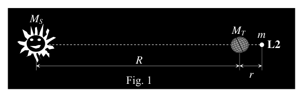Diagrama alineación Sol–Tierra–L2 (Fig. 1)

Topic: Gravitation, Astrophysics, Newtonian Mechanics Metodi: Newton’s Law of Gravitation, Kepler’s Laws, Approximation & Series Expansion, Dimensional Analysis Competenze: Mathematical Modeling, Physical Reasoning Objects: Satellite, Planet, Star Fonte: Testo (PDF) — p.5

P2.- La misión Planck Surveyor

Planck Surveyor è la terza missione del programma scientifico Horizon 2000 dell’Agenzia spaziale europea. Il programma ha lo scopo di rilevare anisotropie nel fondo cosmico di microonde in tutto il cielo, con una risoluzione e sensibilità senza precedenti. Il satellite Planck sarà una fonte di dati molto preziosa, con cui si tenteranno di verificare le teorie attuali sull’universo primitivo e le origini delle strutture cosmiche. Questo satellite è stato lanciato dalla Guayana francese il 14 maggio 2009, propulsato da un razzo Ariane 5.

Il satellite descriverà un’orbita praticamente circolare attorno al Sole, con la particolarità che, in ogni momento, tale satellite, la Terra e il Sole saranno allineati, il che implica che la velocità angolare di rotazione del satellite attorno al Sole, $\omega$, deve essere uguale a quella della Terra. Questa ultima caratteristica (sima $\omega$ che la Terra) è proprio quella che definisce i cosiddetti punti di Lagrange del sistema SolTerra. Si può dimostrare che esistono cinque di questi punti (chiamati $L_1$ a $L_5$). In particolare, il satellite Planck si trova al punto $L_2$, che è allineato al Sole e alla Terra, come mostrato in figura 1. A questo punto non arriva mai la radiazione diretta del Sole, permanentemente eclipsata dalla Terra.

a) Supponendo che l’orbita della Terra intorno al Sole sia circolare, determina la velocità angolare di rotazione $\omega$ in funzione della costante di gravità, $G$, la massa del Sole, $M_S$, e il raggio di orbita, $R$.

b) Il satellite Planck, che è sottoposto alle attrazioni gravitazionali del Sole e della Terra, deve descrivere un’orbita con la stessa $\omega$ della Terra, ma con un raggio maggiore, $R+r$, dove $r$ è la distanza dalla Terra al punto $L_2$. Tenendo questo in considerazione, ottieni l’equazione che devono soddisfare $R$, $r$, $M_S$ e $M_T$ (massa della Terra). Esprimere questa equazione in funzione dei coefficienti $M_T/M_S$ e $r/R$.

c) In pratica, $r\ll R$ e $M_T\ll M_S$, che consentono di avvicinarsi all’equazione di cui al paragrafo precedente. Verifica che può essere ridotto a $r\approx R{\left(\frac{M_T}{3M_S}\right)}^{1/3}$ (Nota: per effettuare approssimazioni può essere utile sapere che $\epsilon \ll 1\Rightarrow (1+\epsilon {)}^n\approx 1+n\epsilon$.)

d) Calcola il valore della distanza $r$ utilizzando i seguenti dati:

• Accelerazione della gravità sulla superficie terrestre: $g=9,8{\text{ m/s}}^2$
• Radio della Terra: $R_T=6,4\times 10^6\text{ m}$
• Periodo di rivoluzione della Terra intorno al Sole: $T=1\text{ an˜o}$

e) Come detto all’inizio, ci sono cinque punti di Lagrange. Otro de ellos, el $L_3$, está a una distancia del Sol prácticamente igual al radio $R$ de la órbita de la Tierra. Dove credi che possa essere questo punto? La distancia entre $L_3$ y el Sol, ¿será algo mayor o algo menor que $R$? Raziona le tue risposte.

Diagramma di allineamento SolTerraL2 (Fig. 1)

Topic: Gravitation, Astrophysics, Newtonian Mechanics Metodi: Newton’s Law of Gravitation, Kepler’s Laws, Approximation & Series Expansion, Dimensional Analysis Competenze: Mathematical Modeling, Physical Reasoning Objects: Satellite, Planet, Star Fonte: Testo (PDF) — p.5

P2.- La misión Planck Surveyor

Planck Surveyor is the third mission of the European Space Agency’s Horizon 2000 science programme. The programme aims to detect anisotropy in the cosmic microwave background throughout the sky, with unprecedented resolution and sensitivity. The Planck satellite will be a valuable source of data to try to test current theories about the early universe and the origins of cosmic structures. This satellite was launched from French Guiana on May 14, 2009, powered by an Ariane 5 rocket.

The satellite will describe an orbit practically circular around the Sun, with the particularity that at all times such a satellite, the Earth and the Sun will be aligned, which implies that the angular rotation speed of the satellite around the Sun, $\omega$, must be equal to that of the Earth. This last feature (the same $\omega$ as the Earth) is precisely what defines the so-called Lagrange points of the Solar system Earth. It can be shown that there are five of these points (called $L_1$ to $L_5$). In particular, the Planck satellite will be located at the $L_2$ point, which is aligned with the Sun and Earth, as shown in Figure 1. At this point, direct radiation from the Sun never reaches, permanently eclipsed by the Earth.

(a) Assuming that the Earth’s orbit around the Sun is circular, it determines the angular rotation speed $\omega$ in terms of the gravitational constant, $G$, the mass of the Sun, $M_S$, and the radius of the orbit, $R$.

(b) The Planck satellite, which is subject to the gravitational pulls of the Sun and the Earth, must describe an orbit with the same $\omega$ as the Earth but with a greater radius, $R+r$, where $r$ is the distance from the Earth to the point $L_2$. With this in mind, get the equation that they must meet $R$, $r$, $M_S$ and $M_T$ (Earth mass). Express this equation in terms of the $M_T/M_S$ and $r/R$ coefficients.

(c) In practice, $r\ll R$ and $M_T\ll M_S$, which allows approximations to be made in the equation in the previous paragraph. It is possible to reduce the $r\approx R{\left(\frac{M_T}{3M_S}\right)}^{1/3}$ (Note: To make approximations, it may be useful to know that $\epsilon \ll 1\Rightarrow (1+\epsilon {)}^n\approx 1+n\epsilon$.)

(d) Calculate the distance $r$ using the following data:

• Gravitational acceleration at the Earth’s surface: $g=9,8{\text{ m/s}}^2$
• Radio of the Earth: $R_T=6,4\times 10^6\text{ m}$
• Period of revolution of the Earth around the Sun: $T=1\text{ an˜o}$

(e) As stated in the introduction, there are five Lagrange points. Otro de ellos, el $L_3$, está a una distancia del Sol prácticamente igual al radio $R$ de la órbita de la Tierra. Where do you think this point might be? La distancia entre $L_3$ y el Sol, ¿será algo mayor o algo menor que $R$? Reason your answers.

Diagrama alineación Sol–Tierra–L2 (Fig. 1)

Topic: Gravitation, Astrophysics, Newtonian Mechanics Metodi: Newton’s Law of Gravitation, Kepler’s Laws, Approximation & Series Expansion, Dimensional Analysis Competenze: Mathematical Modeling, Physical Reasoning Objects: Satellite, Planet, Star Fonte: Testo (PDF) — p.5

P3.- Líneas de campo electrostático

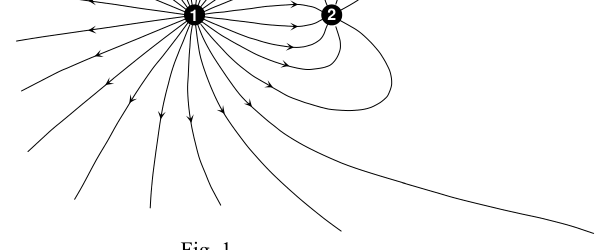
Un campo electrostático puede representarse gráficamente mediante sus líneas de fuerza (o de campo). El número de líneas que “nacen” o “mueren” en una carga es proporcional a la magnitud de dicha carga. (La expresión matemática de esta idea constituye el teorema de Gauss). El campo eléctrico en cada punto es tangente a la línea de fuerza que pasa por dicho punto, y su intensidad es proporcional a la densidad de líneas (número de líneas por unidad de superficie) que hay en su entorno.

En la figura 1 se muestran las líneas de fuerza que describen el campo electrostático generado por dos cargas puntuales, $q_1$ y $q_2$, separadas una distancia $d$.

a) Justifica de qué signo es cada una de las cargas.

b) ¿Cuál es su magnitud relativa, $q_1/q_2$?

c) Razona, con la mayor precisión posible, en qué punto o puntos del plano de la figura 1 el campo electrostático $\vec{E}$ creado por ambas cargas es nulo.

d) Determina en qué punto o puntos del plano de dicha figura es nulo el potencial electrostático creado por las dos cargas.

Considera ahora la distribución de cargas puntuales representada en la figura 2, con $Q_1=6\mu \text{C}$, $Q_2=-2\mu \text{C}$ y $d=4\text{ cm}$.

e) Calcula el potencial electrostático, $V$, y el campo eléctrico, $\vec{E}$, en el punto $A$ de la figura, situado a 3 cm de $Q_1$ y a 1 cm de $Q_2$.

f) Dibuja las líneas de fuerza para esta distribución de cargas.

$\text{Dato: }K=\frac{1}{4\pi {\epsilon }_0}=9\times 10^9{\text{ N⋅m}}^2/{\text{C}}^2$

Líneas de campo dos cargas q1, q2 (Fig. 1)

Distribución Q1, A, Q2 con distancia d (Fig. 2)

Topic: Electrostatics, Geometric Optics Metodi: Coulomb’s Law, Gauss’s Law, Electric Potential Method, Superposition Principle Competenze: Diagrammatic Reasoning, Physical Reasoning Objects: Point Charge Fonte: Testo (PDF) — p.9

P3.- Linee di campo elettrostatico

Un campo elettrostatico può essere rappresentato graficamente attraverso le sue linee di forza (o di campo). Il numero di linee che “nascono” o “moriscono” in un carico è proporzionale alla grandezza di tale carico. (L’espressione matematica di questa idea costituisce il teorema di Gauss). Il campo elettrico in ogni punto è tangente alla linea di forza che passa attraverso tale punto, e la sua intensità è proporzionale alla densità di linee (numero di linee per unità di superficie) che vi è nel suo ambiente.

La figura 1 mostra le linee di forza che descrivono il campo elettrostatico generato da due cariche puntate, $q_1$ e $q_2$, separate da una distanza $d$.

a) giustifica il segno di ciascuna delle cariche.

b) Qual è la sua magnitudine relativa, $q_1/q_2$?

c) Raziona, con la massima precisione possibile, in quale punto o punti del piano di figura 1 il campo elettrostatico $\vec{E}$ creato da entrambe le cariche è nullo.

d) Determina a quale punto o punti del piano di tale figura il potenziale elettrostatico creato dalle due cariche è nullo.

Considera ora la distribuzione di carichi puntuali rappresentata nella figura 2, con $Q_1=6\mu \text{C}$, $Q_2=-2\mu \text{C}$ e $d=4\text{ cm}$.

e) Calcola il potenziale elettrostatico, $V$, e il campo elettrico, $\vec{E}$, nel punto $A$ della figura, situato a 3 cm da $Q_1$ e a 1 cm da $Q_2$.

(f) Disegna le linee di forza per questa distribuzione di cariche.

$\text{Dato: }K=\frac{1}{4\pi {\epsilon }_0}=9\times 10^9{\text{ N⋅m}}^2/{\text{C}}^2$

Line di campo due cariche q1, q2 (Fig. 1)

Distribuzione Q1, A, Q2 con distanza d (Fig. 2)*

Topic: Electrostatics, Geometric Optics Metodi: Coulomb’s Law, Gauss’s Law, Electric Potential Method, Superposition Principle Competenze: Diagrammatic Reasoning, Physical Reasoning Objects: Point Charge Fonte: Testo (PDF) — p.9

The following is the list of the components of the test:

An electrostatic field can be represented graphically by its force (or field) lines. The number of lines that ‘be born’ or ‘die’ on a load is proportional to the magnitude of that load. (The mathematical expression of this idea is Gauss’ theorem.) The electric field at each point is tangent to the force line passing through that point, and its intensity is proportional to the density of lines (number of lines per unit area) in its environment.

Figure 1 shows the lines of force describing the electrostatic field generated by two point charges, $q_1$ and $q_2$, separated by a distance $d$.

(a) Justify the sign of each of the charges.

(b) What is its relative magnitude, $q_1/q_2$?

(c) Reason, as accurately as possible, at which point or points in the plane of Figure 1 the electrostatic field $\vec{E}$ created by both charges is zero.

(d) Determine at which point or points in the plane of the figure the electrostatic potential created by the two charges is zero.

Consider now the spot load distribution as shown in Figure 2, with $Q_1=6\mu \text{C}$, $Q_2=-2\mu \text{C}$ and $d=4\text{ cm}$.

(e) Calculate the electrostatic potential, $V$, and the electric field, $\vec{E}$, at the $A$ point in the figure, located 3 cm from $Q_1$ and 1 cm from $Q_2$.

(f) Draw the lines of force for this load distribution.

$\text{Dato: }K=\frac{1}{4\pi {\epsilon }_0}=9\times 10^9{\text{ N⋅m}}^2/{\text{C}}^2$

The following table shows the values of the values of the values of the values of the values of the values of the values of the values of the values of the values of the values of the values of the values of the values of the values of the values of the values of the values of the values of the values of the values of the values of the values of the values of the values of the values of the values of the values of the values of the values of the values of the values of the values of the values of the values of the values of the values of the values of the values of the values of the values of the values of the values of the values of the values of the values of the values of the values of the values of the values of the values of the values of the values of the values of the values of the values of the values of the values of the values of the values of the values of the values of the values of the values of the values of the values of the values of the values of the values of the values of the values of the values of the values of the values of the values of the values of the values of the values of the values of the values of the values of the values of the values of the values of the values of the values of the values of the values of the values of the values of the values of the values of the values of the values of the values of the values of the values of the values of the values of the values of the values of the values of the values of the values of the first of the first of the first of the first of the first of the first of the first of the first of the first of the first of the first of those values of the first. 1)*

The following table shows the distribution of Q1, A, Q2 with distance d (Fig. 2)*

Topic: Electrostatics, Geometric Optics Metodi: Coulomb’s Law, Gauss’s Law, Electric Potential Method, Superposition Principle Competenze: Diagrammatic Reasoning, Physical Reasoning Objects: Point Charge Fonte: Testo (PDF) — p.9