Spagna 2025

Ejercicio 1. (1 punto) Determina la velocidad angular de la Tierra $Ω$ alrededor del Sol en función de la masa del Sol $M_{S}$ y la distancia Sol-Tierra $ℓ$ . A continuación, obtén su valor numérico utilizando $G = 6, 7 \cdot 1 0^{- 11} Nm^{2} / kg^{2}$ , $M_{S} = 2 \cdot 1 0^{30} kg$ , $M_{T} = 6 \cdot 1 0^{24} kg$ y $ℓ = 1 UA = 1, 5 \cdot 1 0^{8} km$ . Existen un total de 5 puntos de Lagrange denominados $L_{1}$ , $L_{2}$ , $L_{3}$ , $L_{4}$ y $L_{5}$ , ver figura 1. Estos puntos son de especial importancia en astrofísica dado que en ellos se pueden colocar satélites, telescopios y sondas espaciales con un gasto mínimo de combustible debido a sus propiedades de equilibrio y estabilidad. Figura 1: Puntos de Lagrange del sistema Sol-Tierra. Los puntos $L_{1}$ , $L_{2}$ y $L_{3}$ se encuentran en la línea que une el Sol y la Tierra, mientras que $L_{4}$ y $L_{5}$ se encuentran sobre la órbita terrestre formando sendos triángulos equiláteros con lado común el segmento que une al Sol con la Tierra.

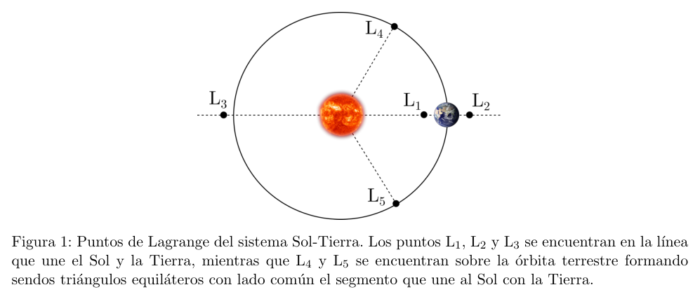Punti di Lagrange sistema Sole-Terra

Topic: Gravitation, Astrophysics, Newtonian Mechanics Metodi: Newton’s Law of Gravitation, Kepler’s Laws, Kinematic Equations Competenze: Mathematical Modeling, Physical Reasoning, Unit Conversion Objects: Planet, Star, Satellite Fonte: Testo (PDF) — p.5

Esercizio 1. (1 punto) Determina la velocità angolare della Terra $Ω$ attorno al Sole in funzione di massa del Sole $M_{S}$ e distanza Sole-Terra $ℓ$ . Quindi, otteni il suo valore numerico usando $G = 6, 7 \cdot 1 0^{- 11} Nm^{2} / kg^{2}$ , $M_{S} = 2 \cdot 1 0^{30} kg$ , $M_{T} = 6 \cdot 1 0^{24} kg$ y $ℓ = 1 UA = 1, 5 \cdot 1 0^{8} km$ . Esistono un totale di 5 punti Lagrange denominati $L_{1}$ , $L_{2}$ , $L_{3}$ , $L_{4}$ e $L_{5}$ , vedi figura 1. Questi punti Sono di particolare importanza in astrofisica, dato che possono essere posizionati satelliti, telescopi. e sonde spaziali con un consumo minimo di carburante a causa delle loro proprietà di equilibrio e Stabilità. Figura 1: Punti di Lagrange del sistema Sole-Terra. I punti $L_{1}$ , $L_{2}$ e $L_{3}$ sono nella linea che unisce il Sole e la Terra, mentre $L_{4}$ e $L_{5}$ si trovano sull’orbita terrestre formando Si formano triangoli equilati con un lato comune che unisce il Sole alla Terra.

Punti di Lagrange sistema Sole-Terra

Exercise one. (1 point) Determines the angular velocity of the Earth $Ω$ around the Sun as a function of The mass of the Sun $M_{S}$ and the Sun-Earth distance $ℓ$ . Then get its numerical value using $G = 6, 7 \cdot 1 0^{- 11} Nm^{2} / kg^{2}$ , $M_{S} = 2 \cdot 1 0^{30} kg$ , $M_{T} = 6 \cdot 1 0^{24} kg$ y $ℓ = 1 UA = 1, 5 \cdot 1 0^{8} km$ . There are a total of 5 Lagrange points named $L_{1}$ , $L_{2}$ , $L_{3}$ , $L_{4}$ and $L_{5}$ , see Figure 1. These points They are of particular importance in astrophysics because they can be used to place satellites, telescopes, and other astronomical instruments. and space probes with minimum fuel consumption due to their balancing properties and The Commission is not prepared to take any further action. Figure 1: Lagrange points of the Sun-Earth system. The points $L_{1}$ , $L_{2}$ and $L_{3}$ are in the line which unites the Sun and the Earth, while $L_{4}$ and $L_{5}$ lie above the Earth’s orbit forming equilateral triangles with a common side the segment that connects the Sun to the Earth.

The Commission has also adopted a proposal for a regulation on the protection of the environment.

Ejercicio 2. (1.5 puntos) Explica cualitativamente por qué los puntos de Lagrange se deben encontrar necesariamente en el plano que contiene a la órbita terrestre.

Parte uno Para un observador $O$ sobre la superficie terrestre (es decir, un observador que gira con velocidad angular $Ω$ alrededor del Sol), un cuerpo situado en cualquier punto de Lagrange se encontrará en reposo. Por ello, a partir de ahora trabajaremos desde este punto de vista. Para este observador, una partícula de masa $m$ en reposo no solo se ve sometida a la fuerza gravitatoria, sino que por el hecho de estar girando aparece la denominada fuerza centrífuga. Esta fuerza apunta en la dirección del vector que une al eje de giro con la partícula y tiene módulo $F = m R Ω^{2}$ , donde $R$ es la distancia entre de la partícula al Sol.

Topic: Gravitation, Rotational Dynamics, Astrophysics Metodi: Free-Body Diagram, Newton’s Law of Gravitation, Physical Modeling Competenze: Physical Reasoning, Diagrammatic Reasoning Objects: Planet, Star Fonte: Testo (PDF) — p.5

Esercizio 2. (1.5 punti) Spiega qualitativamente perché i punti di Lagrange devono necessariamente trovarsi sul piano che contiene l’orbita terrestre.

Parte uno Per un osservatore $O$ sulla superficie terrestre (cioè un osservatore che gira a velocità angular $Ω$ alrededor del Sol), un cuerpo situado en cualquier punto de Lagrange se encontrará en Riposo. Per questo, da ora in poi, lavoreremo da questo punto di vista. Per questo osservatore, una La particella di massa $m$ a riposo non solo è sottoposta alla forza gravitazionale, ma è di essere in rotazione appare la cosiddetta forza centrifugante. Questa forza punta nella direzione del Vettore che lega l’asse di rotazione alla particella e ha modulo $F = m R Ω^{2}$ , dove $R$ è la distanza

E’ il sole.

Exercise two. (1.5 points) Qualitatively explains why Lagrange points must necessarily be found in the plane containing Earth orbit.

Part one For an observer $O$ on the earth’s surface (i.e. an observer spinning at speed) angle $Ω$ around the Sun), a body located at any point in Lagrange will be found at I’m going to rest. We shall therefore work from this point of view. For this observer, one The mass particle $m$ at rest is not only subjected to gravitational force but also to the fact that If you are spinning, you will see the so-called centrifugal force. This force points in the direction of the vector that links the spin axis to the particle and has the module $F = m R Ω^{2}$ , where $R$ is the distance It’s going from the particle to the sun.

Ejercicio 3. (1 punto) Escribe la 2ª Ley de Newton vista por $O$ para la Tierra y demuestra que la suma de fuerzas es cero, es decir, que la Tierra se encuentra en reposo para $O$ . A continuación, vamos a determinar de manera aproximada la posición de los puntos de Lagrange $L_{1}$ , $L_{2}$ y $L_{3}$ , es decir los que se encuentran sobre la línea que une al Sol y la Tierra.

Topic: Newtonian Mechanics, Rotational Dynamics, Gravitation Metodi: Free-Body Diagram, Vector Decomposition, Newton’s Law of Gravitation Competenze: Mathematical Modeling, Diagrammatic Reasoning Objects: Planet, Star Fonte: Testo (PDF) — p.6

Esercizio 3. (1 punto) Escribe la 2ª Ley de Newton vista por $O$ para la Tierra y demuestra que la la somma delle forze è zero, cioè la Terra è in riposo per $O$ . Quindi, determineremo in modo approssimativo la posizione dei punti di Lagrange $L_{1}$ , $L_{2}$ e $L_{3}$ , cioè quelli che si trovano sulla linea che unisce il Sole e la Terra.

Exercise three. (1 punto) Escribe la 2ª Ley de Newton vista por $O$ para la Tierra y demuestra que la The sum of forces is zero, that is, the Earth is at rest for $O$ . A continuación, vamos a determinar de manera aproximada la posición de los puntos de Lagrange $L_{1}$ , $L_{2}$ and $L_{3}$ , that is, those located above the line connecting the Sun and Earth.

Ejercicio 4. (2 puntos) (a) Realiza un diagrama de fuerzas para una partícula prueba sobre los puntos $L_{1}$ , $L_{2}$ y $L_{3}$ para justificar cualitativamente que son puntos de equilibrio. (b) Para cada uno de ellos, discute que ocurriría si perturbas ligeramente la posición de la partícula en la dirección Tierra-Sol: ¿la partícula tiende a alejarse (equilibrio inestable) o a retornar al punto de Lagrange (equilibrio estable)? Sean $ℓ_{1}$ , $ℓ_{2}$ y $ℓ_{3}$ las distancia entre el Sol y los puntos $L_{1}$ , $L_{2}$ y $L_{3}$ , respectivamente.

Topic: Gravitation, Newtonian Mechanics, Rotational Dynamics Metodi: Free-Body Diagram, Physical Modeling, Approximation & Series Expansion Competenze: Physical Reasoning, Diagrammatic Reasoning Objects: Planet, Star Fonte: Testo (PDF) — p.6

Esercizio 4. (2 punti) (a) Realizza un diagramma delle forze per una particella di prova sui punti $L_{1}$ , $L_{2}$ e $L_{3}$ per la qualitativa di giustificare che sono punti di equilibrio. (b) Per ciascuno di essi, discutete cosa accadrebbe se disturbate leggermente la posizione della particella in direzione Terra-Sol: la particella tende a allontanarsi (equilibrio instabile) o a tornare al punto di Lagrange (equilibrio stabile)? Sono $ℓ_{1}$ , $ℓ_{2}$ e $ℓ_{3}$ le distanze tra il Sole e i punti $L_{1}$ , $L_{2}$ e $L_{3}$ , rispettivamente.

Exercise four. (two points) (a) Draw a force diagram for a test particle on the points $L_{1}$ , $L_{2}$ and $L_{3}$ for qualitatively justify that they are balancing points. (b) For each of them, discuss what would happen if you slightly disturbed the position of the particle In the Earth-Sun direction: does the particle tend to move away (unstable equilibrium) or return to the Lagrange point (stable equilibrium)? The distance between the Sun and the points $L_{1}$ , $L_{2}$ and $L_{3}$ shall be $ℓ_{1}$ , $ℓ_{2}$ and $ℓ_{3}$ respectively.

Ejercicio 5. (1.5 puntos) Encuentra las ecuaciones que satisfacen $ℓ_{1}$ , $ℓ_{2}$ y $ℓ_{3}$ en función de $M_{S}$ , $M_{T}$ y $ℓ$ (no hace falta que las resuelvas). Extra: A partir de los valores numéricos de $M_{S}$ y $M_{T}$ , demuestra una (la que quieras) de las siguientes afirmaciones:

La distancia entre la Tierra y $L_{1}$ es menor al 2 % de la distancia Tierra-Sol.
La distancia Tierra- $L_{2}$ es menor al 2 % de la distancia Tierra-Sol.
La distancia Sol- $L_{3}$ es aproximadamente igual (con una diferencia inferior al 1 %), pero mayor que la distancia Sol-Tierra. Pista: Recuerda que, por el Teorema de Bolzano, una función continua $f$ definida en un intervalo $[a, b]$ y que satisface $f (a) \cdot f (b) < 0$ necesariamente se anula en al menos un punto del intervalo $(a, b)$ .

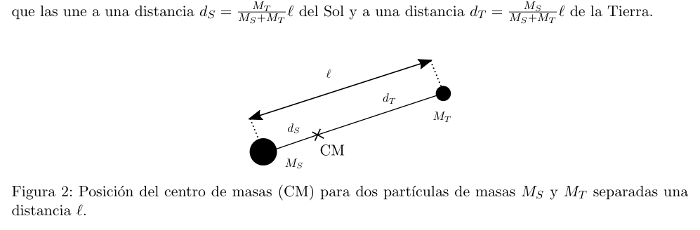
Parte dos Como ya hemos visto, además de los puntos $L_{1}$ , $L_{2}$ y $L_{3}$ , existen otros dos puntos de equilibrio denominados $L_{4}$ y $L_{5}$ . Para determinar la posición de estos puntos, en la segunda parte del problema abandonaremos la visión simplista de que la Tierra orbita alrededor del Sol. En realidad, ambas describen una órbita circular alrededor del centro de masas (CM) del sistema, situado sobre el segmento que las une a una distancia $d_{S} = \frac{M _{T}}{M _{S} + M _{T}} ℓ$ del Sol y a una distancia $d_{T} = \frac{M _{S}}{M _{S} + M _{T}} ℓ$ de la Tierra.

Figura 2: Posición del centro de masas (CM) para dos partículas de masas $M_{S}$ y $M_{T}$ separadas una distancia $ℓ$ . Ejercicio 7. (1 punto) Determina numéricamente la posición del centro de masas del sistema Sol- Tierra. ¿A cuánta distancia de cada uno de los astros se encuentra? Dado que el radio del Sol es de unos $7 \cdot 1 0^{5} km$ , ¿cómo de realista es asumir que la Tierra orbita alrededor del Sol? En este segundo acercamiento más realista el módulo de la fuerza centrífuga sigue siendo $F = m R Ω^{2}$ , pero $R$ y $Ω$ cambian respecto a la Parte 1. Ahora, $R$ es la distancia de la partícula al centro de masas y $Ω^{2} = G (M_{S} + M_{T}) / ℓ^{3}$ . Ejercicio 8. (2 puntos) Demuestra que los puntos $L_{4}$ y $L_{5}$ se encuentran formando sendos triángulos equiláteros con lado común la recta que une al Sol con la Tierra. Ejercicio extra. Imagina que eres científica o científico de la Agencia Espacial Europea (ESA) y te encargan poner en órbita las siguientes misiones. ¿En qué puntos de Lagrange situarías los siguientes satélites y por qué?

Telescopio espacial James Webb, sustituto del telescopio Hubble, cuya misión es observar los objetos más distantes del cosmos.
Observatorio Solar Heliosférico (SOHO), destinado a proporcionar datos solares en tiempo real.
Satélite Planck, diseñado para estudiar las tenues irregularidades del fondo cósmico de microondas, una radiación muy débil que inunda el universo.

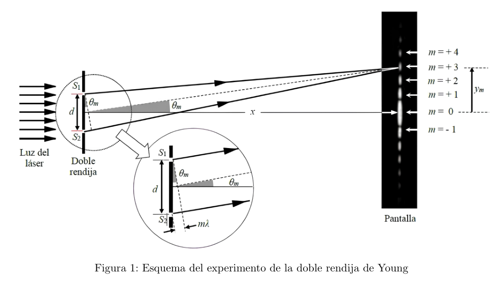
Problema Experimental Objetivo Comprobar el carácter ondulatorio de la luz y determinar la longitud de onda de una luz láser. Introducción La naturaleza de la luz ha sido objeto de discusión desde la antigüedad. Si nos situamos en épocas más recientes cabe señalar dos interpretaciones encontradas: Isaac Newton (1643-1727) sostenía que la luz estaba constituida por partículas, mientras que Christiaan Huygens (1629-1695) defendía su carácter ondulatorio. En 1807, Thomas Young dio a conocer lo que se conoce como el experimento de la doble rendija. Se trataba de un experimento que, a pesar de su sencillez, establecía de forma irrefutable la naturaleza ondulatoria de la luz. Las conclusiones del experimento eran tan sólidas que existieron pocas dudas acerca de esa interpretación a lo largo del siglo XIX. El nacimiento de la hipótesis cuántica en 1900 de la mano de Max Planck y su posterior aplicación en 1905 para interpretar el efecto fotoeléctrico por parte de Albert Einstein obligaron a reconsiderar la naturaleza de la luz; pero esa ya es otra historia… Figura 1: Esquema del experimento de la doble rendija de Young

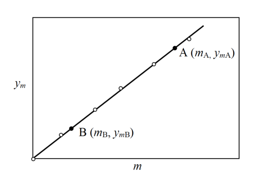
Fundamento teórico La luz monocromática de un puntero láser incide sobre dos rendijas $S_{1}$ y $S_{2}$ paralelas muy próximas, cuya separación es $d$ (ver Figura 1). Estas rendijas se convierten en fuentes secundarias de luz que se encuentran en fase. Sobre una pantalla situada a una distancia $x$ de las dos rendijas (con $x ≫ d$ ) llega luz procedente de ellas. Si la luz tiene naturaleza ondulatoria, en las posiciones de la pantalla en que la diferencia de caminos ópticos es un número entero de longitudes de onda $(λ)$ , se producirá interferencia constructiva. Por lo tanto, se cumple que $sin θ_{m} = \frac{mλ}{d} . (1)$ Por otra parte, entre la posición de cualquier máximo de luz en la pantalla $(y_{m})$ medida desde la posición del máximo central y la distancia desde la doble rendija a la pantalla $(x)$ existe la siguiente relación $tan θ_{m} = \frac{y _{m}}{x} . (2)$ Como las distancias $y_{m}$ son muy pequeñas comparadas con la distancia $x$ se puede considerar que $sin θ_{m} \approx tan θ_{m}$ . Con esta aproximación, a partir de las expresiones (1) y (2) puede escribirse $\frac{y _{m}}{x} = \frac{mλ}{d} . (3)$ De acuerdo con la expresión (3), si se representan gráficamente las posiciones de los máximos de interferencias $(y_{m})$ en ordenadas, frente a los correspondientes órdenes $(m)$ en abscisas, se obtendrá un conjunto de puntos que pueden ajustarse a una línea recta, cuya pendiente será $λ x / d$ . Con el valor de la pendiente y conocidos los valores de $x$ y de $d$ , puede obtenerse el de la longitud de onda $λ$ . Una vez trazada la recta que mejor se ajusta a los datos experimentales, para determinar la pendiente pueden tomarse dos puntos de la recta A y B suficientemente separados (ver Figura a la izquierda), cuyas coordenadas son $A = (m_{A}, y_{m, A})$ y $B = (m_{B}, y_{m, B})$ . La pendiente de la recta es $\frac{λ x}{d} = \frac{y _{m, A} - y _{m, B}}{m _{A} - m _{B}} . (4)$

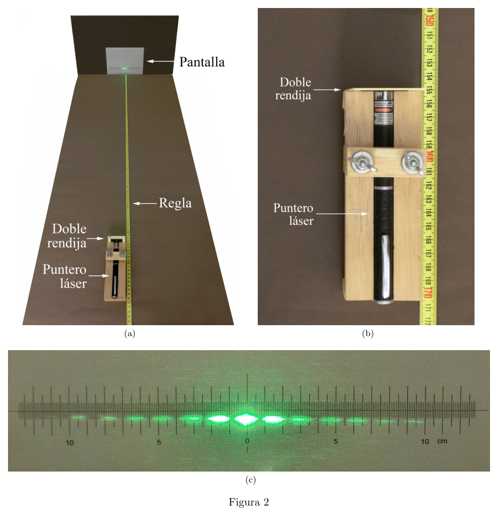
Procedimiento Experimental Se ha montado el dispositivo mostrado en la Figuras 2a y 2b. Un puntero láser ilumina una doble rendija montada en un pequeño marco, con una distancia entre las rendijas $d = 52 μ m$ . La distancia (en centímetros) de la doble rendija a la pantalla $(x)$ en la que se observan las interferencias se muestra en la Figura 2b. (a) (b) (c) Figura 2

Determina la longitud de onda del láser mediante los siguientes pasos:

En la pantalla hay una escala de medida sobre la que se proyectan las interferencias (ver Figura 2c). La interferencia de orden $m = 0$ está situada en el 0 de la escala, con las interferencias de orden $\pm 1$ , $\pm 2$ , etc. a ambos lados. Mide las sucesivas distancias $y_{m}$ que puedas reconocer y traslada los resultados a una tabla como la que se muestra a continuación. (2 puntos) m $y_{m}$ (cm) 0 … 1 … 2 … … …
Representa gráficamente los valores de $y_{m}$ (en ordenadas) frente a los de $m$ (en abscisas) y traza la recta que mejor se ajusta a los puntos experimentales. (3 puntos)
A partir de los dos puntos de la recta que hayas elegido y aplicando la expresión (4) halla el valor de la pendiente de la recta. (3 puntos)
Con el valor hallado para la pendiente y los valores de $x$ (ver Figura 2b) y $d$ , determina la longitud de onda de la luz. (2 puntos)

Topic: Gravitation, Astrophysics, Wave Optics Metodi: Approximation & Series Expansion, Newton’s Law of Gravitation, Interference & Diffraction Analysis Competenze: Mathematical Modeling, Experimental Data Analysis, Graph Linearization Objects: Planet, Star, Slit, Screen Fonte: Testo (PDF) — p.6

Figure

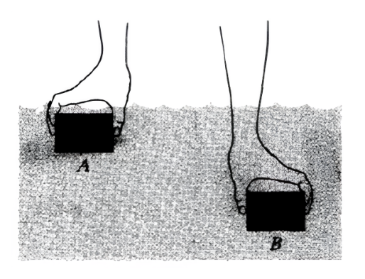
p.3 — Blocchi A e B sommersi in acqua

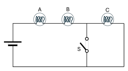
p.4 — Circuito tre lampade con interruttore S

p.7 — Centro di massa tra due masse MS e MT

p.8 — Schema esperimento doppia fenditura Young

p.9 — Retta dei massimi di interferenza

p.10 — Apparato doppia fenditura e pantalla (a,b,c)

Esercizio 5. (1.5 punti) Trova le equazioni che soddisfano $ℓ_{1}$ , $ℓ_{2}$ e $ℓ_{3}$ in funzione di $M_{S}$ , $M_{T}$ e $ℓ$ (non è necessario risolverle). Extra: a partire dai valori numerici di $M_{S}$ e $M_{T}$ , dimostrare uno (qualsiasi) dei seguenti: affermazioni:

La distanza tra la Terra e $L_{1}$ è inferiore al 2% della distanza Terra-Sol.
La distanza Terra- $L_{2}$ è inferiore al 2% della distanza Terra-Solo.
La distanza Sol- $L_{3}$ è approssimativamente uguale (con una differenza inferiore all’1%) ma maggiore che la distanza Sole-Terra. Costruttore: Ricorda che, dal Teorema di Bolzano, una funzione continua $f$ definita in un intervallo $[a, b]$ e che soddisfa $f (a) \cdot f (b) < 0$ è necessariamente annullato almeno in un punto dell’intervallo $(a, b)$ .

Parte due Come abbiamo già visto, oltre ai punti $L_{1}$ , $L_{2}$ e $L_{3}$ , ci sono altri due punti di equilibrio denominati $L_{4}$ e $L_{5}$ . Per determinare la posizione di questi punti, nella seconda parte del problema abbandoneremo la visione simplista che la Terra orbita intorno al Sole. In realtà, entrambi descrivono un’orbita circolare intorno al centro di massa (CM) del sistema, situato sul segmento che li unisce a una distanza $d_{S} = \frac{M _{T}}{M _{S} + M _{T}} ℓ$ dal Sole e a una distanza $d_{T} = \frac{M _{S}}{M _{S} + M _{T}} ℓ$ dalla Terra.

Figura 2: Posizione del centro di massa (CM) per due particelle di massa $M_{S}$ e $M_{T}$ separate da una Distanza $ℓ$ . Esercizio 7. (1 punto) Determina numericamente la posizione del centro di massa del sistema solare. Terra. A che distanza si trova ogni stella? Dato che il raggio del Sole è di unos $7 \cdot 1 0^{5} km$ , ¿cómo de realista es asumir que la Tierra orbita alrededor del Sol? In questo secondo approccio più realistico il modulo di forza centrifuge è ancora $F = m R Ω^{2}$ , se la parte 1 è stata modificata, il $R$ e $Ω$ sono modificati rispetto alla parte 1. Ora, $R$ è la distanza della particella al centro di massa y $Ω^{2} = G (M_{S} + M_{T}) / ℓ^{3}$ . Esercizio 8. (2 punti) Dimostra che i punti $L_{4}$ e $L_{5}$ sono in forma di sentieri triangolari equilaterali con lato comune la retta che collega il Sole alla Terra. Esercizio extra. Immaginate di essere uno scienziato o uno scienziato dell’Agenzia Spaziale Europea (ESA) e di Incomando di mettere in orbita le seguenti missioni. In quali punti di Lagrange si trovano i seguenti satelliti e perché?

Il telescopio spaziale James Webb, sostituto del telescopio Hubble, ha come missione osservare le oggetti più lontani del cosmo.
Observatorio solare eliosferico (SOHO), destinato a fornire dati solari in tempo reale.
Il satellite Planck, progettato per studiare le sottili irregolarità del fondo cosmico di microonde, una radiazione molto debole che inonda l’universo.

Problema sperimentale Obiettivo Verificare il carattere ondulatorio della luce e determinare la lunghezza d’onda di una luce laser. Introduzione La natura della luce è stata oggetto di discussione fin dall’antichità. Se ci troviamo in un’epoca più La luce è una fonte di energia, che è stata inventata nel 1643 e che è stata inventata nel 1727 era costituita da particelle, mentre Christiaan Huygens (1629-1695) difendeva il suo carattere

l’ondulazione. Nel 1807, Thomas Young pubblicò quello che è noto come l’esperimento della doppia
La spazzatura. Si trattava di un esperimento che, nonostante la sua semplicità, stabilisce in modo irrefutabile la natura ondulatoria della luce. Le conclusioni dell’esperimento erano così solide che esistevano nel corso del XIX secolo. La nascita dell’ipotesi quantistica nel 1900 da parte di Max Planck e la sua successiva applicazione nel 1905 per interpretare l’effetto Albert Einstein ha costretto a riconsiderare la natura della luce, ma questa è già la luce che E’ un’altra storia… Figura 1: Schema dell’esperimento della doppia fessura di Young

Fondamento teorico La luce monocromatica di un puntatore laser incide su due spazi $S_{1}$ e $S_{2}$ molto vicini, di cui la separazione è $d$ (vedere figura 1). Queste spazzature diventano fonti secondarie di luce che sono in fase. Su uno schermo situato a $x$ distanza dalle due spazzature (con $x ≫ d$ ) e la luce viene da loro. Se la luce è ondulatoria, nelle posizioni dello schermo se la differenza di percorsi ottici è un numero intero di lunghezze d’onda $(λ)$ , si produrrà interferenza costruttiva. Si tratta pertanto di: $sin θ_{m} = \frac{mλ}{d} . (1)$ Inoltre, tra la posizione di qualsiasi massimo di luce sullo schermo $(y_{m})$ misurata dal la posizione della massima centrale e la distanza dal doppio fisso allo schermo $(x)$ è la seguente: Relazione $tan θ_{m} = \frac{y _{m}}{x} . (2)$ Poiché le distanze $y_{m}$ sono molto piccole rispetto alla distanza $x$ si può considerare che $sin θ_{m} \approx tan θ_{m}$ . Con questo approccio, a partire dalle espressioni (1) e (2) si può scrivere $\frac{y _{m}}{x} = \frac{mλ}{d} . (3)$ In base all’espressione (3), se si rappresentano graficamente le posizioni dei massimi di interferenza $(y_{m})$ in ordinati, rispetto ai corrispondenti ordini $(m)$ in abscissi, si ottiene un un insieme di punti che possono essere fissati su una linea retta, la cui pendenza sarà $λ x / d$ . Con il valore di se la pendenza è nota e i valori $x$ e $d$ sono noti, si può ottenere quello della lunghezza d’onda $λ$ . Una volta tracciato il tratto che si adatta meglio a dati sperimentali, per determinare la pendenza può essere preso due punti di La linea A e B sono sufficientemente separate (vedi Figura a sinistra), le cui coordinate sono $A = (m_{A}, y_{m, A})$ y $B = (m_{B}, y_{m, B})$ . La pendenza della retta è $\frac{λ x}{d} = \frac{y _{m, A} - y _{m, B}}{m _{A} - m _{B}} . (4)$

Procedura sperimentale Il dispositivo mostrato nelle figure 2a e 2b è stato montato. Un puntatore laser illumina un doppio spaziatura montata su un piccolo quadro, con una distanza tra le spaziature $d = 52 μ m$ . Distanza (in centimetri) dalla doppia rottura al display $(x)$ in cui si osservano le interferenze è mostrato in Figura 2b. (a) (b) (c) Figura 2

Determina la lunghezza d’onda del laser attraverso i seguenti passaggi:

Sullo schermo c’è una scala di misura su cui vengono proiettate le interferenze (vedere Figura 2c). L’interferenza di ordine $m = 0$ è situata al 0 della scala, con le interferenze di ordine $\pm 1$ , $\pm 2$ , ecc. - Da entrambi i lati. Misura le distanze successive $y_{m}$ che puoi riconoscere e trasmette i risultati in una tabella come la seguente. (2 punti) m $y_{m}$ (cm) 0 … 1 … 2 … … …
Rappresenta graficamente i valori di $y_{m}$ (ordinati) rispetto a quelli di $m$ (abcissi) e traccia la retta che meglio si adatta ai punti sperimentali. (3 punti)
A partire dai due punti della retta che hai scelto e applicando l’espressione (4) trovi il valore della pendenza della retta. (3 punti)
Con il valore trovato per la pendenza e i valori $x$ (vedi figura 2b) e $d$ , determina la lunghezza d’onda della luce. (2 punti)

Figurare

**p.3 ** Blocchi A e B sommersi in acqua

**p.4 ** Circuito a tre lampadine con interruttore S

p.7 — Centro di massa tra due masse MS e MT

p.8 — Schema esperimento doppia fenditura Young

**p.9 ** Retta dei massimi di interferenza

p.10 Apparecchio doppio fenditura e schermo (a,b,c)

Exercise five. Find the equations satisfying $ℓ_{1}$ , $ℓ_{2}$ and $ℓ_{3}$ for $M_{S}$ , $M_{T}$ and $ℓ$ (no need to solve them). Extra: From the numerical values of $M_{S}$ and $M_{T}$ , prove one (which you want) of the following: the following statements:

The distance between Earth and $L_{1}$ is less than 2% of the Earth-Sun distance.
The Earth- $L_{2}$ distance is less than 2% of the Earth-Sun distance.
The distance Sol- $L_{3}$ is approximately equal (with a difference of less than 1%) but greater than than the Sun-Earth distance. Note: Remember that, by the Bolzano Theorem, a continuous function $f$ defined in an interval $[a, b]$ and satisfying $f (a) \cdot f (b) < 0$ is necessarily cancelled at least one point in the $(a, b)$ interval.

Part two As we have already seen, in addition to the $L_{1}$ , $L_{2}$ and $L_{3}$ points, there are two other equilibrium points called $L_{4}$ and $L_{5}$ . To determine the position of these points, in the second part of the problem We’ll abandon the simplistic view that the Earth orbits the Sun. In fact, both describe a circular orbit around the center of mass (CM) of the system, located above the segment which connects them to a distance $d_{S} = \frac{M _{T}}{M _{S} + M _{T}} ℓ$ from the Sun and a distance $d_{T} = \frac{M _{S}}{M _{S} + M _{T}} ℓ$ from the Earth.

Figure 2: Position of the centre of mass (CM) for two particles of mass $M_{S}$ and $M_{T}$ separated by one The distance $ℓ$ .

Exercise seven. (1 point) Determines numerically the position of the center of mass of the solar system. Earth. How far away from each of the stars is it? Since the radius of the Sun is from unos $7 \cdot 1 0^{5} km$ , ¿cómo de realista es asumir que la Tierra orbita alrededor del Sol? In this second more realistic approach the centrifugal force module remains $F = m R Ω^{2}$ , pero $R$ y $Ω$ cambian respecto a la Parte 1. Ahora, $R$ es la distancia de la partícula al centro de masas y $Ω^{2} = G (M_{S} + M_{T}) / ℓ^{3}$ . Exercise eight. (2 points) Demonstrates that the $L_{4}$ and $L_{5}$ points are triangular in shape Equilaterals with a common side the straight line that connects the Sun to the Earth. Extreme exercise. Imagine that you are a scientist or a scientist from the European Space Agency (ESA) and you They’re in charge of putting the following missions into orbit. Where on Lagrange would you place the following satellites and why?

The James Webb Space Telescope, which replaced the Hubble Telescope, is the most distant objects in the cosmos.
Heliospheric Solar Observatory (SOHO), intended to provide real-time solar data.
Planck satellite, designed to study the faint irregularities of the cosmic microwave background, a very weak radiation that floods the universe.

The experimental problem Objective Check the wavelength of the light and determine the wavelength of a laser light. The following is the list of the countries of the European Union: The nature of light has been the subject of debate since ancient times. If we are in more times The most recent interpretations are two: Isaac Newton (1643-1727) argued that light is a matter of great importance. It was made up of particles, while Christiaan Huygens (1629-1695) defended its character. The waveform. In 1807, Thomas Young released what is known as the double experiment. The crack. It was an experiment which, despite its simplicity, established irrefutably that the the wavy nature of light. The experiment’s conclusions were so solid that they existed. There was little doubt about that interpretation throughout the 19th century. The birth of the quantum hypothesis in 1900 by Max Planck and its subsequent application in 1905 to interpret the effect The photoelectric effect by Albert Einstein forced us to reconsider the nature of light; but that already It’s another story… Figure 1: Schematic of the Young double-slit experiment

Theoretical basis The monochrome light of a laser pointer hits two very close parallel $S_{1}$ and $S_{2}$ slits, cuya separación es $d$ (ver Figura 1). These slits become secondary sources of light that They’re in phase. On a screen located at a distance $x$ from the two slots (with $x ≫ d$ ) Light comes from them. If the light is wave-like, in the position of the screen where the difference in optical paths is an integer of wavelengths $(λ)$ , it shall be constructive interference. It is therefore true that $sin θ_{m} = \frac{mλ}{d} . (1)$ In addition, between the position of any maximum light on the display $(y_{m})$ measured from the position of the central maximum and distance from the double slit to the screen $(x)$ is as follows: The relationship $tan θ_{m} = \frac{y _{m}}{x} . (2)$ Since the distances $y_{m}$ are very small compared to the distance $x$ it can be considered that $sin θ_{m} \approx tan θ_{m}$ . With this approximation, from the expressions (1) and (2) it can be written $\frac{y _{m}}{x} = \frac{mλ}{d} . (3)$ According to expression (3), if the positions of the interference maxims $(y_{m})$ are represented graphically in ordered, versus the corresponding orders $(m)$ in abscises, a a set of points which can be adjusted to a straight line, the slope of which shall be $λ x / d$ . With the value of The slope and known values of $x$ and $d$ can be obtained for the wavelength $λ$ . Once the straight line is drawn, it fits best. to experimental data, to determine The slope can be taken two points from straight A and B sufficiently separated (see Figure on the left), whose coordinates are $A = (m_{A}, y_{m, A})$ y $B = (m_{B}, y_{m, B})$ . The slope of the straight line is $\frac{λ x}{d} = \frac{y _{m, A} - y _{m, B}}{m _{A} - m _{B}} . (4)$

The Commission shall adopt the following implementing acts: The device shown in Figures 2a and 2b has been installed. A laser pointer lights up a double a small-frame mounted slit, with a distance between the slits $d = 52 μ m$ . The distance (in centimeters) from the double slit to the $(x)$ display where interference is observed In Figure 2b. (a) (b) (c) Figure 2

Determine the laser wavelength by the following steps:

On the screen there is a measurement scale on which interference is projected (see Figure 2c). The interference order $m = 0$ is located at 0 on the scale, with the interferences de orden $\pm 1$ , $\pm 2$ , etc. Both sides. Measure the successive distances $y_{m}$ that you can recognize and The results are then moved to a table like the one shown below. (two points) m $y_{m}$ (cm) 0 … 1 … 2 … … …
Graphically represents the values of $y_{m}$ (in ordered) versus $m$ (in abscises) and traces the strait that best fits the experimental points. (three points)
From the two points of the line you have chosen and applying the expression (4) you find the the value of the slope of the straight line. (three points)
With the value found for the slope and the values of $x$ (see Figure 2b) and $d$ , determine the wavelength of light. (two points)

Figure

p.3 — Blocchi A e B sommersi in acqua

**p.4 ** Three lamp circuit with switch S

p.7 — Centro di massa tra due masse MS e MT

p.8 — Schema esperimento doppia fenditura Young

p.9 — Retta dei massimi di interferenza

p.10 Scratch and screen double apparatus (a,b,c)

Raccolta Gare di Fisica

Esplora

Spagna 2025

Figure

Figure

Figure

Figure

Figure

Figure

Figure

Figure

Figure

Figure

Figure

Figure

Figure

Figurare

Figurare

Figurare

Figurare

Figurare

Figurare

Figurare

Figurare

Figurare

Figurare

Figurare

Figurare

Figurare

Figure

Figure

Figure

Figure

Figure

Figure

Figure

Figure

Figure

Figure

Figure

Figure

Figure

Vista grafico

Indice