Svizzera 2024

Figura B.1: Conduttore piano a massa infinitamente lungo con una carica $Q_1$ in una posizione ${\vec{r}}_1=(x_1,y_1,z_1)=(0,0,d)$.

i. (0.25 pt) Quali sono le condizioni al contorno per il potenziale elettrostatico $V$ di questo sistema?

ii. (1.5 pt) Immaginiamo un secondo sistema fisico con la stessa carica $Q_1$ nella stessa posizione ${\vec{r}}_1$ della Fig. B.1 ma senza il piano conduttore. Il nostro obiettivo è trovare una configurazione con una seconda carica $Q_2$ nella posizione ${\vec{r}}_2$ che abbia le stesse condizioni al contorno della Fig. B.1. Quali dovrebbero essere i valori di $Q_2$ e ${\vec{r}}_2=(x_2,y_2,z_2)$ perché ciò avvenga? Perché?

iii. (1 pt) Utilizzando i risultati precedenti, calcolare il potenziale elettrico $V(x,y,z)$ al di sopra del suolo nel sistema di Fig. B.1 in funzione delle coordinate $(x,y,z)$, della distanza $d$ e della carica $Q_1$. L’espressione può essere lasciata come somma di due termini, non è necessario semplificarla completamente.

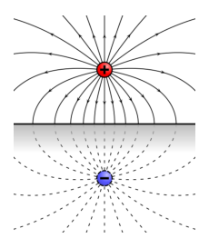
iv. (1.5 pt) Disegnare schematicamente il sistema di conduttori di Fig. B.1 con le linee di campo corrispondenti, assumendo che $Q_1>0$ (in uno schizzo separato, non sul foglio del problema).

Parte C. Carica immagine ad angolo retto (5.5 punti)

Considereremo ora geometrie di conduttori più complesse.

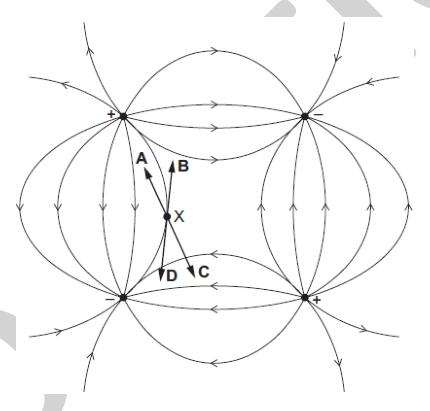
i. (2.5 pt) Consideriamo il sistema mostrato in Fig. C.1. Qual è il numero $N$ di cariche speculari necessarie per riprodurre le condizioni limite del conduttore? Quali sono i loro valori $Q_i$ e le loro posizioni ${\vec{r}}_i=(x_i,y_i,z_i)$ per $i=1,2,\dots ,N$? Perché?

Figura C.1: Due semipiani conduttori infinitamente lunghi messi a terra ad angolo retto con una carica $Q_1$ nella posizione ${\vec{r}}_1=(x_1,y_1,z_1)=(d,0,d)$.

ii. (1 pt) Qual è il potenziale corrispondente $V(x,y,z)$ in funzione delle coordinate $(x,y,z)$, della distanza $d$ e della carica $Q_1$? L’espressione può essere lasciata come somma di $N$ termini, non è necessario semplificarla completamente.

iii. (2 pt) Disegnare schematicamente il sistema carica-mezzo piano-conduttore con le linee di campo corrispondenti, assumendo che $Q_1<0$ (in uno schizzo separato, non sul foglio del problema).

Parte D. Cariche dello specchio circolare (4 punti)

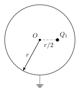
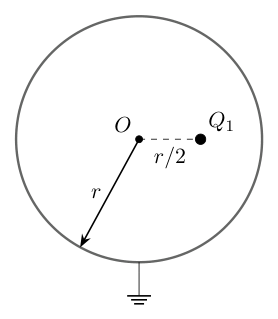
i. (2.5 pt) Consideriamo ora il sistema mostrato in Fig. D.1. Si scopre che è necessaria una sola carica speculare per riprodurre le condizioni al contorno corrispondenti. Qual è il suo valore $Q_2$ e la sua posizione ${\vec{r}}_2=(x_2,y_2,z_2)$?

Suggerimento: si può usare senza prova che un potenziale che soddisfa le condizioni al contorno appropriate nelle posizioni $(r,0,0)$ e $(-r,0,0)$ soddisfa le condizioni al contorno sull’intera sfera.

Figura D.1: Conduttore sferico a massa di raggio $r$ con centro $O$ in posizione ${\vec{r}}_0=(0,0,0)$ e carica $Q_1$ in posizione ${\vec{r}}_1=(x_1,y_1,z_1)=(r/2,0,0)$. Qui vediamo una fetta a $y=0$ della sfera nel piano $xz$.

ii. (1.5 pt) Qual è il potenziale corrispondente $V(x,y,z)$ in funzione delle coordinate $(x,y,z)$, del raggio $r$ e della carica $Q_1$? L’espressione può essere lasciata come somma di due termini, non è necessario semplificarla completamente.

SOLUTION

Problemi lunghi: soluzioni

Problema lungo 2.1: Stabilità di un uovo

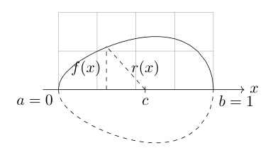
Consideriamo un uovo rappresentato da un solido omogeneo di rivoluzione con profilo $f(x)=\frac{1}{2}\sqrt{x-x^4}$ sul dominio $x\in [a=0,b=1]$. Le unità di lunghezza sono arbitrarie.

Parte A. Centro di gravità e raggio

Il baricentro $c$ di un solido di rivoluzione si trova sul suo asse e può essere calcolato dividendolo in dischi di spessore infinitesimale $dx$ e volume $\pi f^2(x)dx$:

$c=\frac{1}{V}{\int }_a^{b}x\pi f^2(x)dx,$

dove $V$ è il volume del solido.

i. Calcolare $c$ per l’uovo.

Following the idea of splitting the egg into disk-shaped infinitely thin slices, the volume is given by:

$V={\int }_a^b\pi f^2(x)dx.$

Thus for the egg, we have

$c=\frac{{\int }_0^{1}x\frac{1}{4}(x-x^4)dx}{{\int }_0^1\frac{1}{4}(x-x^4)dx}=\frac{{\int }_0^1(x^2-x^5)dx}{{\int }_0^1(x-x^4)dx}=\frac{{\left[\frac{1}{3}{x}^3-\frac{1}{6}{x}^6\right]}_0^1}{{\left[\frac{1}{2}{x}^2-\frac{1}{5}{x}^5\right]}_0^1},$

And finally

$c=\frac{\frac{1}{3}-\frac{1}{6}}{\frac{1}{2}-\frac{1}{5}}=\frac{\frac{1}{6}}{\frac{3}{10}}=\frac{5}{9}.$

ii. Se fosse stato scelto un fattore diverso da $\frac{1}{2}$ nel profilo $f(x)$ dell’uovo, quale sarebbe stato l’impatto sul valore di $c$? Giustificare.

SOLUTION

$c$ wouldn’t change, because the factor (squared) appears both in the numerator and in the denominator of $c$.

This is the same reason why the egg’s density doesn’t play a role, nor does $\pi$.

iii. Trovare un’espressione per il «raggio» $r(x)$ dell’uovo, cioè la distanza tra il baricentro e un punto $(x,f(x))$ sulla superficie dell’uovo. Il risultato deve essere della forma $\sqrt{P(x)}$, dove $P(x)$ è un polinomio.

We can use the Pythagorean theorem:

$r(x)=\sqrt{f^2(x)+(x-c{)}^2},$

and we get

$r(x)=\sqrt{\frac{1}{4}x-\frac{1}{4}{x}^4+x^2+c^2-2xc}=\sqrt{-\frac{1}{4}{x}^4+x^2-\frac{31}{36}x+\frac{25}{81}}.$

Parte B. Intermezzo analitico

Sia $g(x)>0$ una funzione differenziabile strettamente positiva.

i. Espandere $\frac{d\sqrt{g(x)}}{dx}$, la derivata della radice quadrata di $g(x)$.

We can use the generic formula

$\frac{d{g}^n(x)}{dx}=n{g}^{n-1}(x)\frac{dg(x)}{dx}.$

Here we have the case $n=\frac{1}{2}$, so

$\frac{d\sqrt{g(x)}}{dx}=\frac{1}{2\sqrt{g(x)}}\frac{dg(x)}{dx}.$

Full points are given as long as the answer is of the desired final form, even if the generic formula is not explicitly stated.

ii. Dimostrare che il segno di $\frac{d\sqrt{g(x)}}{dx}$ è sempre uguale a quello di $\frac{dg(x)}{dx}$.

$g(x)>0\Rightarrow \sqrt{g(x)}>0\Rightarrow \frac{1}{2\sqrt{g(x)}}>0.$

Thus the factor in front of the derivative does not change the sign, so both will always be equal. This is in particular valid for the case $0$: if the derivative of $g(x)$ is null, so is the derivative of $\sqrt{g(x)}$.

Parte C. Stabilità dell’uovo deposto

Poniamo ora l’uovo su una superficie orizzontale e identifichiamo il punto in cui l’uovo è a contatto con la superficie con la sua coordinata $x$.

SOLUTION

i. Le posizioni $a=0$ e $b=1$ sono posizioni di equilibrio, a causa della simmetria di rivoluzione. Determinare la stabilità di queste due posizioni dall’espressione $r(x)$ trovata in A.iii. e utilizzando il risultato mostrato in B.ii.

To study the stability, we need to compute the derivative of the radius found in A.iii. But we are only interested in its sign, so instead, and according to B.ii., we can compute the derivative of its square, $P(x)$.

$\frac{dP(x)}{dx}=-x^3+2x-\frac{31}{36}.$

For $x=a=0$, ${\frac{dP(x)}{dx}|}_a=-\frac{31}{36}<0$.

This means that all values slightly larger than $a$ lead to a smaller $r^2$, thus also to a smaller $r$. Because $a$ is at the end of the domain, it corresponds to a local maximum of the radius, and therefore $a$ is an instable equilibrium.

For $x=b=1$, ${\frac{dP(x)}{dx}|}_b=-1+2-\frac{31}{36}=\frac{5}{36}>0$.

This means that all values slightly smaller than $b$ lead again to a smaller $r^2$, thus also to a smaller $r$. Because $b$ is at the other end of the domain, it corresponds to a local maximum of the radius, and therefore $b$ is an instable equilibrium as well.

Esiste una posizione $a<s<b$ in cui l’uovo disteso su un fianco è in equilibrio stabile.

ii. Qual è la particolarità di $r(s)$?

It is a local minimum of $r(x)$, and in fact its only minimum.

Give 0.5 point if it is only mentioned that the segment of $r(s)$ is perpendicular to the egg’s surface.

iii. Trovare un’equazione polinomiale per $s$.

The condition for $s$ is that the derivative of the radius is zero.

Again we can use B.ii. and only consider the derivative of $P(x)$.

Thus the equation is

$-s^3+2s-\frac{31}{36}=0.$

SOLUTION

Purtroppo, questa equazione polinomiale non è (facilmente) risolvibile. Cercheremo quindi un’approssimazione utilizzando un’espansione di Taylor.

iv. Scegliere un buon punto di partenza $t$ per lo sviluppo. Giustificate la vostra scelta.

If the egg was symmetric, that is an ellipse, $s$ would be in the center ($\frac{1}{2}$).

The egg is not very dissymmetric, so $t=\frac{1}{2}$ is a good starting point, and easy to comput

conduttore sferico a massa Fig D.1

linee di campo piano conduttore a massa

linee di campo sistema quattro cariche speculari

conduttore sferico Fig D.1 soluzione

Topic: Electrostatics, Electromagnetism Metodi: Electric Potential Method, Symmetry Argument, Coulomb’s Law Competenze: Diagrammatic Reasoning, Mathematical Modeling, Physical Reasoning Objects: Point Charge, Conducting Sphere Fonte: Testo (PDF) — p.14

Figure B.1: Infinite plane conducting surface with a charge $Q_1$ located at position ${\vec{r}}_1=(x_1,y_1,z_1)=(0,0,d)$.

i. (0.25 pt) What are the boundary conditions for the electrostatic potential $V$ of this system?

ii. (1.5 pt) Consider a second physical system with the same charge $Q_1$ located at the same position ${\vec{r}}_1$ as in Figure B.1, but without the conducting plane. Our goal is to find a configuration with a second charge $Q_2$ located at position ${\vec{r}}_2$ such that the boundary conditions match those of Figure B.1. What should be the values of $Q_2$ and ${\vec{r}}_2=(x_2,y_2,z_2)$ for this to happen? Why?

iii. (1 pt) Using the previous results, compute the electric potential $V(x,y,z)$ above the ground in the system of Figure B.1 as a function of coordinates $(x,y,z)$, distance $d$, and charge $Q_1$. The expression may be left as a sum of two terms; full simplification is not required.

iv. (1.5 pt) Sketch schematically the conductor system of Figure B.1 with the corresponding field lines, assuming that $Q_1>0$ (on a separate sketch, not on the problem sheet).

Part C. Image charge at right angle (5.5 points)

We will now consider more complex conductor geometries.

i. (2.5 pt) Consider the system shown in Figure C.1. How many image charges $N$ are required to reproduce the boundary conditions of the conductor? What are their values $Q_i$ and positions ${\vec{r}}_i=(x_i,y_i,z_i)$ for $i=1,2,\dots ,N$? Why?

Figure C.1: Two infinitely long grounded conducting half-planes at right angles with a charge $Q_1$ at position ${\vec{r}}_1=(x_1,y_1,z_1)=(d,0,d)$.

ii. (1 pt) What is the corresponding potential $V(x,y,z)$ as a function of the coordinates $(x,y,z)$, the distance $d$ and the charge $Q_1$? The expression may be left as a sum of $N$ terms, it is not necessary to simplify it completely.

iii. (2 pt) Schematically draw the charge-half-plane-conductor system with the corresponding field lines, assuming that $Q_1<0$ (in a separate sketch, not on the problem sheet).

Part D. Circular mirror charges (4 points)

i. (2.5 pt) Let us now consider the system shown in Fig. D.1. It turns out that only one image charge is needed to reproduce the corresponding boundary conditions. What is its value $Q_2$ and its position ${\vec{r}}_2=(x_2,y_2,z_2)$?

Hint: one may use without proof that a potential satisfying the appropriate boundary conditions at the positions $(r,0,0)$ and $(-r,0,0)$ satisfies the boundary conditions on the entire sphere.

Figure D.1: Grounded spherical conductor of radius $r$ with center $O$ at position ${\vec{r}}_0=(0,0,0)$ and charge $Q_1$ at position ${\vec{r}}_1=(x_1,y_1,z_1)=(r/2,0,0)$. Here we see a slice at $y=0$ of the sphere in the plane $xz$.

ii. (1.5 pt) What is the corresponding potential $V(x,y,z)$ as a function of the coordinates $(x,y,z)$, the radius $r$ and the charge $Q_1$? The expression may be left as a sum of two terms, it is not necessary to simplify it completely.

SOLUTION

Long Problems: Solutions

Long Problem 2.1: Stability of an Egg

Consider an egg represented by a homogeneous solid of revolution with profile $f(x)=\frac{1}{2}\sqrt{x-x^4}$ on the domain $x\in [a=0,b=1]$. Length units are arbitrary.

Part A. Center of gravity and radius

The center of mass $c$ of a solid of revolution lies on its axis and can be computed by dividing it into infinitesimally thin disks of thickness $dx$ and volume $\pi f^2(x)dx$:

$c=\frac{1}{V}{\int }_a^{b}x\pi f^2(x)dx,$

where $V$ is the volume of the solid.

i. Compute $c$ for the egg.

Following the idea of splitting the egg into disk-shaped infinitely thin slices, the volume is given by:

$V={\int }_a^b\pi f^2(x)dx.$

Thus for the egg, we have

$c=\frac{{\int }_0^{1}x\frac{1}{4}(x-x^4)dx}{{\int }_0^1\frac{1}{4}(x-x^4)dx}=\frac{{\int }_0^1(x^2-x^5)dx}{{\int }_0^1(x-x^4)dx}=\frac{{\left[\frac{1}{3}{x}^3-\frac{1}{6}{x}^6\right]}_0^1}{{\left[\frac{1}{2}{x}^2-\frac{1}{5}{x}^5\right]}_0^1},$

And finally

$c=\frac{\frac{1}{3}-\frac{1}{6}}{\frac{1}{2}-\frac{1}{5}}=\frac{\frac{1}{6}}{\frac{3}{10}}=\frac{5}{9}.$

ii. If a different factor than $\frac{1}{2}$ had been chosen in the profile $f(x)$ of the egg, what would have been the impact on the value of $c$? Justify.

SOLUTION

$c$ would not change, because the factor (squared) appears both in the numerator and in the denominator of $c$.

This is the same reason why the egg’s density doesn’t play a role, nor does $\pi$.

iii. Find an expression for the “radius” $r(x)$ of the egg, i.e., the distance between the center of mass and a point $(x,f(x))$ on the egg’s surface. The result must be of the form $\sqrt{P(x)}$, where $P(x)$ is a polynomial.

We can use the Pythagorean theorem:

$r(x)=\sqrt{f^2(x)+(x-c{)}^2},$

and we get

$r(x)=\sqrt{\frac{1}{4}x-\frac{1}{4}{x}^4+x^2+c^2-2xc}=\sqrt{-\frac{1}{4}{x}^4+x^2-\frac{31}{36}x+\frac{25}{81}}.$

Part B. Analytical interlude

Let $g(x)>0$ be a differentiable strictly positive function.

i. Expand $\frac{d\sqrt{g(x)}}{dx}$, the derivative of the square root of $g(x)$.

We can use the generic formula

$\frac{d{g}^n(x)}{dx}=n{g}^{n-1}(x)\frac{dg(x)}{dx}.$

Here we have the case $n=\frac{1}{2}$, so

$\frac{d\sqrt{g(x)}}{dx}=\frac{1}{2\sqrt{g(x)}}\frac{dg(x)}{dx}.$

Full points are awarded as long as the answer is in the required final form, even if the general formula is not explicitly stated.

ii. Prove that the sign of $\frac{d\sqrt{g(x)}}{dx}$ is always equal to that of $\frac{dg(x)}{dx}$.

$g(x)>0\Rightarrow \sqrt{g(x)}>0\Rightarrow \frac{1}{2\sqrt{g(x)}}>0.$

Thus, the factor in front of the derivative does not change the sign, so both will always be equal. This is particularly valid for the case $0$: if the derivative of $g(x)$ is zero, then so is the derivative of $\sqrt{g(x)}$.

Part C. Stability of the deposited egg

Now place the egg on a horizontal surface and identify the point where the egg contacts the surface by its coordinate $x$.

SOLUTION

i. The positions $a=0$ and $b=1$ are equilibrium positions, due to axial symmetry. Determine the stability of these two positions using the expression $r(x)$ obtained in A.iii., and applying the result shown in B.ii.

To study stability, we need to compute the derivative of the radius found in A.iii. However, we are only interested in its sign; therefore, according to B.ii., instead we can compute the derivative of its square, $P(x)$.

$\frac{dP(x)}{dx}=-x^3+2x-\frac{31}{36}.$

For $x=a=0$, ${\frac{dP(x)}{dx}|}_a=-\frac{31}{36}<0$.

This means that all values slightly larger than $a$ lead to a smaller $r^2$, thus also to a smaller $r$. Since $a$ is at the end of the domain, it corresponds to a local maximum of the radius, and therefore $a$ is an unstable equilibrium.

For $x=b=1$, ${\frac{dP(x)}{dx}|}_b=-1+2-\frac{31}{36}=\frac{5}{36}>0$.

This means that all values slightly smaller than $b$ again lead to a smaller $r^2$, thus also to a smaller $r$. Since $b$ is at the other end of the domain, it corresponds to a local maximum of the radius, and therefore $b$ is an unstable equilibrium as well.

There exists a position $a<s<b$ at which the egg lying on its side is in stable equilibrium.

ii. What is special about $r(s)$?

It is a local minimum of $r(x)$, and in fact its only minimum.

Give 0.5 point if it is only mentioned that the segment of $r(s)$ is perpendicular to the egg’s surface.

iii. Find a polynomial equation for $s$.

The condition for $s$ is that the derivative of the radius is zero.

Again we can use B.ii. and only consider the derivative of $P(x)$.

Thus the equation is

$-s^3+2s-\frac{31}{36}=0.$

SOLUTION

Unfortunately, this polynomial equation is not (easily) solvable. We will therefore seek an approximation using a Taylor expansion.

iv. Choose a good starting point $t$ for the expansion. Justify your choice.

If the egg were symmetric, that is an ellipse, $s$ would be at the center ($\frac{1}{2}$).

The egg is not very asymmetric, so $t=\frac{1}{2}$ is a good starting point, and easy to compute.

conducting sphere with mass Figure D.1

field lines, plane conducting surface with mass

field lines, system of four symmetric charges

conducting sphere Figure D.1 solution

e i termini di ordine superiore.

We can start by rewriting the right-hand side of the previous answer in a way that we can use the given Taylor expansion:

${\left(\frac{P_0+h_A}{P_0+h_C}\right)}^{\gamma }={\left(1+\frac{h_A}{P_0}\right)}^{\gamma }{\left(1+\frac{h_C}{P_0}\right)}^{-\gamma }$

Applying the Taylors expansion then gives (keeping only terms linear in $\frac{h_A}{P_0}$ and $\frac{h_C}{P_0}$)

${\left(\frac{P_0+h_A}{P_0+h_C}\right)}^{\gamma }\approx \left(1+\gamma \frac{h_A}{P_0}\right)\left(1-\gamma \frac{h_C}{P_0}\right)\approx 1+\gamma \frac{h_A-h_C}{P_0}.$

We end up with

$\frac{P_0+h_A}{P_0}=1+\gamma \frac{h_A-h_C}{P_0}.$

iv. Utilizzando i risultati precedenti, esprimere l’indice adiabatico $\gamma$ in funzione di $h_A$ e $h_C$.

Isolating $\gamma$ we find

$\gamma =\frac{h_A}{h_A-h_C}.$

v. Calcolare numericamente l’indice adiabatico $\gamma$ a partire dalle misure fornite.

Using the given numerical values for $P_0$, $P_0+h_A$ and $h_C$, one finds

$\gamma =\frac{780.31-766.50}{780.31-766.50-3.61}\approx \mathrm{1.35.}$

vi. Dal teorema di equipartizione, è possibile ricavare che $C_V=\frac{f}{2}R$ e $C_P=\frac{f+2}{2}R$, dove $f$ è il numero di gradi di libertà consentiti per le molecole del gas. Il gas qui studiato ha $f=5$ gradi di libertà. Qual è la differenza relativa tra i valori teorici e quelli sperimentali dell’indice adiabatico $\gamma$?

Using the definition of $\gamma$ we find $\gamma =\frac{f+2}{f}=\frac{7}{5}=1.4$. This gives a relative difference $\frac{{\gamma }_{th}-{\gamma }_{exp}}{{\gamma }_{th}}=3.6\%$.

vii. Quali potrebbero essere le ragioni di questa differenza?

If at least two of the following reasons is mentioned, or any other meaningful potential reasson is mentioned, then the full points are obtained.

The discrepancy could come from: the statistical uncertainty in the measurements, a systematic uncertainty due to a wrong assumption (the process $A\to B$ might not be fully adiabatic, the change of volume due to the pressure changes in the manometer might not be negligible, the initial compression might not be fully isothermic, …), etc.

SOLUTION

Problema lungo 2.3: Carica immagine

Un problema molto comune in elettrostatica è quello di determinare il potenziale elettrico di un sistema composto da cariche puntiformi e conduttori di varia forma. In questo esercizio svilupperemo un metodo, il cosiddetto metodo della carica immagine, per semplificare notevolmente tali problemi nei casi con una simmetria appropriata. In questo esercizio consideriamo il sistema di unità SI.

Parte A. Potenziale elettrico e conduttori

In questa prima parte parleremo delle gabbie di Faraday.

i. Scrivere il potenziale elettrico $V$ dovuto a una carica puntiforme $q$ in funzione della distanza $r$ dalla carica.

The potential is given by $V(r)=\frac{1}{4\pi {\epsilon }_0}\frac{q}{r}$.

ii. Scrivere il potenziale elettrico $V$ dovuto a $N$ cariche puntiformi $q_i$, $i\in 1,2,\dots ,N$, in funzione delle distanze $r_i$ da ciascuna carica $q_i$.

The total potential is given by the sum of the individual potentials: $V=\frac{1}{4\pi {\epsilon }_0}\sum _{i=1}^N\frac{q_i}{r_i}$.

iii. Considerate la situazione mostrata in Fig. B.1. Che cosa si può dire del potenziale elettrico sulla superficie del materiale conduttore collegato a terra?

As we have a grounded conductor, the potential on the surface must vanish, so $V=0$ on the conductor.

iv. Durante un temporale, è più sicuro rimanere in auto o stare all’aperto? Perché? Argomentate utilizzando la risposta alla domanda precedente.

It is safer to stay in one’s car, because the metallic hull of the car is a grounding conducting surface for which $V=0$ holds such that its inside is protected against lightning.

Parte B. Carica immagine con un conduttore piano

Consideriamo nuovamente la situazione illustrata nella Fig. B.1. L’obiettivo di questa parte è determinare il potenziale elettrico in qualsiasi punto al di sopra del piano. A tale scopo, è possibile utilizzare un trucco che semplifica notevolmente la situazione. L’idea è quella di introdurre una carica immaginaria «specchio» per riprodurre le condizioni al contorno poste dal materiale conduttore.

In elettrostatica, se due sistemi fisici hanno potenziali con le stesse condizioni al contorno, le due situazioni sono fisicamente equivalenti.

Quindi, per determinare il potenziale elettrico di questo sistema, vorremmo trovare un altro sistema più semplice per descrivere il suo potenziale.

Figura B.1: Conduttore piano a massa infinitamente lungo con una carica $Q_1$ in una posizione ${\vec{r}}_1=(x_1,y_1,z_1)=(0,0,d)$.

SOLUTION

i. Quali sono le condizioni al contorno per il potenziale elettrostatico $V$ di questo sistema?

As seen in the previous part, the potential must satisfy $V=0$ on the grounded conducting surface.

ii. Immaginiamo un secondo sistema fisico con la stessa carica $Q_1$ nella stessa posizione ${\vec{r}}_1$ della Fig. B.1 ma senza il piano conduttore. Il nostro obiettivo è trovare una configurazione con una seconda carica $Q_2$ nella posizione ${\vec{r}}_2$ che abbia le stesse condizioni al contorno della Fig. B.1. Quali dovrebbero essere i valori di $Q_2$ e ${\vec{r}}_2=(x_2,y_2,z_2)$ perché ciò avvenga? Perché?

By symmetry, we can expect the mirror charge to lie at position ${\vec{r}}_2=(0,0,-d)$.

If the mirror charge lies at $(x_2,y_2,z_2)=(0,0,-d)$ we can check that picking $Q_2=-Q_1$ indeed satisfies the boundary conditions.

Indeed, this must be the case by symmetry. One could also check it explicitly using the result from A.ii.

iii. Utilizzando i risultati precedenti, calcolare il potenziale elettrico $V(x,y,z)$ al di sopra del suolo nel sistema di Fig. B.1 in funzione delle coordinate $(x,y,z)$, della distanza $d$ e della carica $Q_1$. L’espressione può essere lasciata come somma di due termini, non è necessario semplificarla completamente.

The resulting potential in the charge-plane conductor system must be the same as the charge-mirror charge system, so we obtain for $\vec{r}=(x,y,z)$

$V(\vec{r})=\frac{1}{4\pi {\epsilon }_0}\left[\frac{Q_1}{\sqrt{x^2+y^2+(z-d{)}^2}}-\frac{Q_1}{\sqrt{x^2+y^2+(z+d{)}^2}}\right].$

The solution could be written in a different form as long as the potential is written explicitly as a function of the required quantities.

iv. Disegnare schematicamente il sistema di conduttori di Fig. B.1 con le linee di campo corrispondenti, assumendo che $Q_1>0$ (in uno schizzo separato, non sul foglio del problema).

The drawing should qualitatively look like the upper half of the following image. The lower half should contain no field lines.

https://commons.wikimedia.org/wiki/File:VFPt_imagecharge_plane_horizontal_plusminus.svg

SOLUTION

The field lines should flow from the positive charge to the conductor.

The field lines should stop at the level of the conductor.

The field lines at the level of the conductor should be perpendicular to its surface.

Parte C. Carica immagine ad angolo retto

Considereremo ora geometrie di conduttori più complesse.

i. Consideriamo il sistema mostrato in Fig. C.1. Qual è il numero $N$ di cariche speculari necessarie per riprodurre le condizioni limite del conduttore? Quali sono i loro valori $Q_i$ e le loro posizioni ${\vec{r}}_i=(x_i,y_i,z_i)$ per $i=1,2,\dots ,N$? Perché?

Figura C.1: Due semipiani conduttori infinitamente lunghi messi a terra ad angolo retto con una carica $Q_1$ nella posizione ${\vec{r}}_1=(x_1,y_1,z_1)=(d,0,d)$.

We want the potential to vanish on the conductor plates.

By symmetry considerations, we can convince ourselves that the mirror charges should lie at the positions ${\vec{r}}_2=(-d,0,d)$, ${\vec{r}}_3=(-d,0,-d)$ and ${\vec{r}}_4=(d,0,-d)$.

Similarly, we can expect to have $Q_2=Q_4$.

After some trial and error, one can notice that the choice $Q_2=Q_4=-Q_1$ and $Q_3=Q_1$ leads to a vanishing potential on the conducting plates.

Indeed, by saying that $r_i$ is the distance from the position $\vec{r}$ to the charge $i$, we have

$V(\vec{r})=\frac{1}{4\pi {\epsilon }_0}\left(\frac{Q_1}{r_1}-\frac{Q_1}{r_2}+\frac{Q_1}{r_3}-\frac{Q_1}{r_4}\right).$

On the vertical plate, we have $r_1=r_2$ and $r_3=r_4$ such that indeed $V=0$. On the horizontal plate we have $r_1=r_4$ and $r_2=r_3$ so we also have a vanishing potential.

A more explicit computation making less explicit use of symmetries, or a more implicit reasoning with the symmetries is fine as long as the reasoning is corr

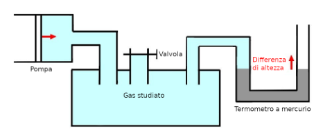schema apparato Clément-Desormes pompa valvola manometro

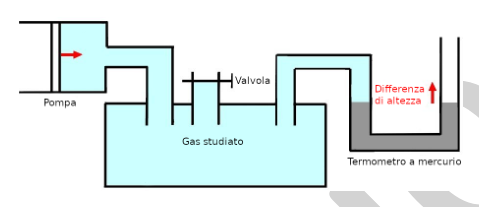schema Clément-Desormes soluzione

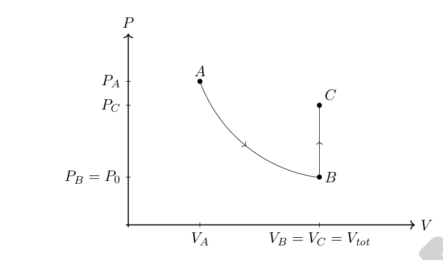diagramma P-V esperimento A B C

Topic: Thermodynamics, Kinetic Theory Metodi: Approximation & Series Expansion, Ideal Gas Law, Experimental Data Analysis Competenze: Experimental Data Analysis, Mathematical Modeling, Physical Reasoning Objects: Point Charge, Manometer, Gas Fonte: Testo (PDF) — p.23

Figure

Figure

Figure

Figure

Figure

Figure

Figure

Figure

Figure

Figure

Figure

Figure

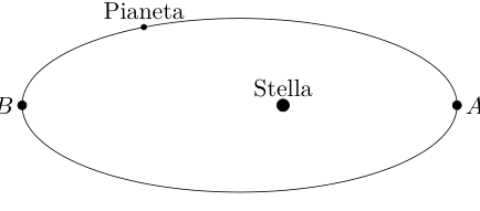
p.4 — orbita ellittica pianeta-stella

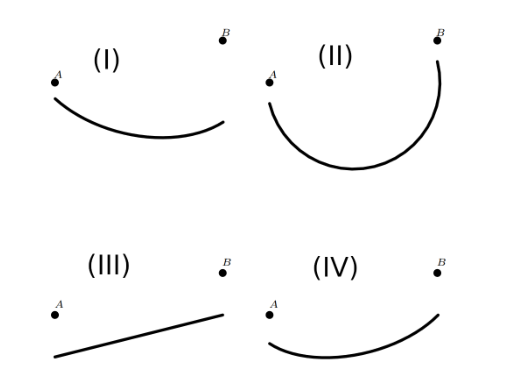
p.4 — quattro traiettorie I-IV corda-carrucola

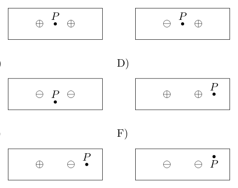
p.6 — configurazioni A-F cariche puntiformi campo E

p.6 — circuito con batterie resistori corrente

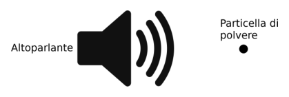
p.6 — altoparlante e particella di polvere

p.11 — profilo uovo f(x) r(x) baricentro c

p.11 — uovo su superficie orizzontale a=0 b=1

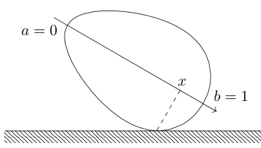
p.18 — uovo su superficie soluzione equilibrio

and higher-order terms.

We can begin by rewriting the right-hand side of the previous answer in a form suitable for applying the given Taylor expansion:

${\left(\frac{P_0+h_A}{P_0+h_C}\right)}^{\gamma }={\left(1+\frac{h_A}{P_0}\right)}^{\gamma }{\left(1+\frac{h_C}{P_0}\right)}^{-\gamma }$

Applying the Taylor expansion then yields (retaining only terms linear in $\frac{h_A}{P_0}$ and $\frac{h_C}{P_0}$)

${\left(\frac{P_0+h_A}{P_0+h_C}\right)}^{\gamma }\approx \left(1+\gamma \frac{h_A}{P_0}\right)\left(1-\gamma \frac{h_C}{P_0}\right)\approx 1+\gamma \frac{h_A-h_C}{P_0}.$

We thus obtain

$\frac{P_0+h_A}{P_0}=1+\gamma \frac{h_A-h_C}{P_0}.$

iv. Using the previous results, express the adiabatic index $\gamma$ as a function of $h_A$ and $h_C$.

Isolating $\gamma$, we find

$\gamma =\frac{h_A}{h_A-h_C}.$

v. Compute numerically the adiabatic index $\gamma$ based on the provided measurements.

Using the given numerical values for $P_0$, $P_0+h_A$ and $h_C$, one finds

$\gamma =\frac{780.31-766.50}{780.31-766.50-3.61}\approx \mathrm{1.35.}$

vi. From the equipartition theorem, it is possible to deduce that $C_V=\frac{f}{2}R$ and $C_P=\frac{f+2}{2}R$, where $f$ is the number of allowed degrees of freedom for gas molecules. The gas studied here has $f=5$ degrees of freedom. What is the relative difference between the theoretical and experimental values of the adiabatic index $\gamma$?

Using the definition of $\gamma$, we find $\gamma =\frac{f+2}{f}=\frac{7}{5}=1.4$. This yields a relative difference $\frac{{\gamma }_{th}-{\gamma }_{exp}}{{\gamma }_{th}}=3.6\%$.

vii. What could be the reasons for this discrepancy?

If at least two of the following reasons are mentioned, or any other meaningful potential reason is mentioned, then full points are awarded.

The discrepancy could come from: the statistical uncertainty in the measurements, a systematic uncertainty due to a wrong assumption (the process $A\to B$ might not be fully adiabatic, the change of volume due to the pressure changes in the manometer might not be negligible, the initial compression might not be fully isothermal, …), etc.

SOLUTION

Problem 2.3: Image Charge

A very common problem in electrostatics is determining the electric potential of a system composed of point charges and conductors of various shapes. In this exercise we will develop a method, called the image charge method, to greatly simplify such problems in cases with appropriate symmetry. In this exercise we use SI units.

Part A. Electric potential and conductors

In this first part we will discuss Faraday cages.

i. Write the electric potential $V$ due to a point charge $q$ as a function of the distance $r$ from the charge.

The potential is given by $V(r)=\frac{1}{4\pi {\epsilon }_0}\frac{q}{r}$.

ii. Write the electric potential $V$ due to $N$ point charges $q_i$, $i\in 1,2,\dots ,N$, as a function of the distances $r_i$ from each charge $q_i$.

The total potential is given by the sum of the individual potentials: $V=\frac{1}{4\pi {\epsilon }_0}\sum _{i=1}^N\frac{q_i}{r_i}$.

iii. Consider the situation shown in Fig. B.1. What can be said about the electric potential on the surface of the grounded conducting material?

Since we have a grounded conductor, the potential on its surface must vanish, so $V=0$ holds on the conductor.

iv. During a thunderstorm, is it safer to stay inside a car or remain outdoors? Why? Argue using the answer to the previous question.

It is safer to stay in one’s car, because the metallic hull of the car is a grounding conducting surface for which $V=0$ holds such that its interior is protected against lightning.

Part B. Image charge with a planar conductor

We again consider the situation illustrated in Fig. B.1. The goal of this part is to determine the electrostatic potential at any point above the plane. To achieve this, it is possible to use a trick that greatly simplifies the situation. The idea is to introduce an imaginary “mirror” charge in order to reproduce the boundary conditions imposed by the conducting material.

In electrostatics, if two physical systems have potentials satisfying the same boundary conditions, then the two situations are physically equivalent.

Therefore, to determine the electrostatic potential of this system, we wish to find another simpler system that describes its potential.

Figure B.1: An infinitely long grounded planar conductor with a charge $Q_1$ located at position ${\vec{r}}_1=(x_1,y_1,z_1)=(0,0,d)$.

SOLUTION

i. What are the boundary conditions for the electrostatic potential $V$ of this system?

As seen in the previous part, the potential must satisfy $V=0$ on the grounded conducting surface.

ii. Imagine a second physical system with the same charge $Q_1$ at the same position ${\vec{r}}_1$ as in Fig. B.1, but without the conducting plane. Our goal is to find a configuration with a second charge $Q_2$ at position ${\vec{r}}_2$ such that it satisfies the same boundary conditions as in Fig. B.1. What should be the values of $Q_2$ and ${\vec{r}}_2=(x_2,y_2,z_2)$ for this to happen? Why?

By symmetry, we expect the mirror charge to be located at position ${\vec{r}}_2=(0,0,-d)$.

If the mirror charge is placed at $(x_2,y_2,z_2)=(0,0,-d)$, we can verify that choosing $Q_2=-Q_1$ indeed satisfies the boundary conditions.

Indeed, this must be true by symmetry. One could also verify it explicitly using the result from A.ii.

iii. Using the previous results, calculate the electric potential $V(x,y,z)$ above ground in the system of Fig. B.1 as a function of coordinates $(x,y,z)$, distance $d$, and charge $Q_1$. The expression may be left as a sum of two terms; it is not necessary to fully simplify it.

The resulting potential in the charge-conductor plane system must be identical to that of the charge-mirror charge system, so we obtain for $\vec{r}=(x,y,z)$

$V(\vec{r})=\frac{1}{4\pi {\epsilon }_0}\left[\frac{Q_1}{\sqrt{x^2+y^2+(z-d{)}^2}}-\frac{Q_1}{\sqrt{x^2+y^2+(z+d{)}^2}}\right].$

The solution could be expressed in a different form, as long as the potential is explicitly written as a function of the required quantities.

iv. Sketch schematically the conductor system in Fig. B.1 with corresponding field lines, assuming $Q_1>0$ (on a separate sketch, not on the problem sheet).

The drawing should qualitatively resemble the upper half of the following image. The lower half should contain no field lines.

https://commons.wikimedia.org/wiki/File:VFPt_imagecharge_plane_horizontal_plusminus.svg

SOLUTION

The field lines should originate from the positive charge and terminate on the conductor.

The field lines should end at the surface of the conductor.

The field lines at the surface of the conductor should be perpendicular to its surface.

Part C. Charge near a right-angled corner

We will now consider more complex conductor geometries.

i. Consider the system shown in Fig. C.1. How many mirror charges $N$ are required to reproduce the boundary conditions on the conductor? What are their values $Q_i$ and positions ${\vec{r}}_i=(x_i,y_i,z_i)$ for $i=1,2,\dots ,N$? Why?

Figure C.1: Two infinitely long grounded conducting half-planes arranged at a right angle, with a charge $Q_1$ located at position ${\vec{r}}_1=(x_1,y_1,z_1)=(d,0,d)$.

We require the potential to vanish on the conductor plates.

By symmetry considerations, we can convince ourselves that the mirror charges should be located at positions ${\vec{r}}_2=(-d,0,d)$, ${\vec{r}}_3=(-d,0,-d)$ and ${\vec{r}}_4=(d,0,-d)$.

Similarly, we can expect to have $Q_2=Q_4$.

After some trial and error, one can notice that the choice $Q_2=Q_4=-Q_1$ and $Q_3=Q_1$ results in a vanishing potential on the conducting plates.

Indeed, by denoting $r_i$ as the distance from position $\vec{r}$ to the charge $i$, we have

$V(\vec{r})=\frac{1}{4\pi {\epsilon }_0}\left(\frac{Q_1}{r_1}-\frac{Q_1}{r_2}+\frac{Q_1}{r_3}-\frac{Q_1}{r_4}\right).$

On the vertical plate, we have $r_1=r_2$ and $r_3=r_4$ such that indeed $V=0$. On the horizontal plate we have $r_1=r_4$ and $r_2=r_3$ so that the potential also vanishes.

A more explicit computation making less explicit use of symmetries, or a more implicit reasoning using symmetries, is acceptable as long as the reasoning is correct.

Clément-Desormes apparatus diagram: pump, valve, manometer

Clément-Desormes experiment solution diagram

P-V diagram of experiment: points A, B, C

Figure

Figure

Figure

Figure

Figure

Figure

Figure

Figure

Figure

Figure

Figure

Figure

p.4 — elliptical orbit of planet-star system

p.4 — four trajectories I–IV for mass-string-pulley system

p.6 — configurations A–F of point charges and corresponding electric field E

p.6 — circuit with batteries, resistors, and current flow

p.6 — loudspeaker and dust particle

p.11 — egg-shaped profile: f(x), r(x), center of mass c

p.11 — egg on horizontal surface: case a=0, b=1

p.18 — egg on surface: solution for equilibrium condition