APhO 2008 — Teorica

Tea Ceremony and Physics of Bubbles

The tea ceremony is traditional in Asia. One of the important steps in preparation of tea is the boiling of fresh water when bubbles appear inside. Bubbles are familiar from daily life and occupy an important role in physics, chemistry, medicine and technology. Nevertheless, their behavior is often surprising and unexpected and, in many cases, still not understood.

At room temperature the pure water is saturated with gas. With increasing temperature the excess pressure of dissolved gas $P_{gb}$ increases, the dissolved air is liberated and air bubbles (ABs) appear at the bottom and walls of teakettle (Fig. 2). For pure water the wettability is sufficient and an AB represents a truncated sphere with radius $R_{ab}$ and with unwetted foundation with radius $r_{ab}<<R_{ab}$. At more heating ABs expand and by reaching certain sizes can detach from the bottom (Fig. 3), flow up to the water surface and burst there. The vapor bubbles (VBs) appear when the water temperature at the bottom reaches the critical value $T_{cr}^b=T_{cr0}^b=100{}^{\circ }C$ at which the pressure of the saturated vapor exceeds the external pressure. The vapor production increases ten times, the VBs expand and detach from the bottom. VB may be considered consisting only of vapor. If the water is heated sufficiently, the uprising VB continue to swell, reach the surface and burst. Else, water is not heated enough in the higher layers and there exits a vertical strong temperature gradient. By reaching relatively cold layers of water VB collapse in the volume of water (Fig. 4). This causes the induced degassing - strong oscillations and a considerable amount of dissolved air is released in the form of microscopic air bubbles (MAB). This can generate ultrasonic vibrations.

The main stages of the bubble evolution during the boiling process are:

• the appearance and growth of AB at the bottom and walls, their transmutation into VB;
• the detachment and uprising of VB, their disappearance in the water volume or at the surface;
• the appearance of MAB in the water volume and their uprising to the surface.

This theoretical description is in good agreement with modern experiments. Particularly, an interesting noise analysis experiment (NAE, Ural State University, Ekaterinburg) for the boiling water was performed. Highly sensitive microphones attached to wide-band amplifiers and brought to an electric teakettle have detected three main origins of noises:

1. ABs detachments from the bottom before boiling (generate oscillations with ${\nu }_1\sim 100$ Hz);
2. VB’s collapses in the volume of water (generate oscillations with ${\nu }_2\sim 1$ kHz);
3. MAB’s appearances under the water surface (generate oscillations with ${\nu }_3\sim 35$ kHz to 60 kHz).

Hints

1) It is well known that a small bubble rises along a rectilinear path and a laminar flow is observed - water flows easy and layer-wise (see Fig.1). Then, the Stokes formula describes the dissipative force for a particle moving with slow velocity $v_{slow}$: $F_d=6\pi {\eta }_w{R}_b{v}_{slow}$

In contrast to this picture, when relatively large bubbles lift to the surface, it disturbs the surrounding water; cavitation hollows appear behind and the turbulent flow is observed (see Fig.1). In this case a part of the kinetic energy of an uprising bubble transfers into the dissipative work.

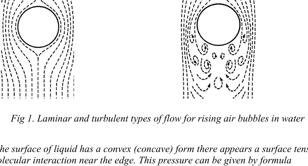Fig. 1. Laminar and turbulent types of flow for rising air bubbles in water.

2) When the surface of liquid has a convex (concave) form there appears a surface tension force due to molecular interaction near the edge. This pressure can then be given by formula $\Delta P=\frac{2\sigma }{R}$ where $\sigma$ is the surface tension coefficient (unit = N/m), the force coming to unit of length of surface, $R$ is the radius of surface curvature.

3) When dealing with a short process with characteristic duration time "$\tau$", its inverse value may be considered as a characteristic frequency $\nu =\frac{1}{\tau }$. Use this definition for calculating the noise frequencies.

Useful data

• $P_a=1.016\cdot 10^5$ [Pa] - atmospheric pressure,
• ${\rho }_w=10^3$ [kg / m³] - water density,
• ${\rho }_{vapor}=0.017$ [kg / m³] - vapor density at T = 293 K; ($\zeta =0.596$ [kg / m³] at T = 373 K)
• $P_{vapor}=0.023\cdot 10^5$ [Pa] - vapor pressure at T = 293 K; ($1.016\cdot 10^5$ [Pa] at T = 373 K)
• $g=9.81$ [m / s²] - acceleration of gravity,
• ${\mu }_{air}=0.029$ [kg / mole] - molecular weight of air,
• $R=8.31$ [J / mole · K] - the gas universal constant,
• $\sigma =0.0725$ [N / m] - surface tension coefficient of water,
• ${\eta }_w=0.3\cdot 10^{-3}$ [Pa · s] - coefficient of viscosity of water,
• H = 10 cm — Water attitude in teakettle.

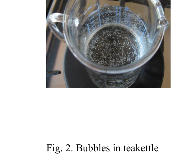Fig. 2. Bubbles in teakettle.

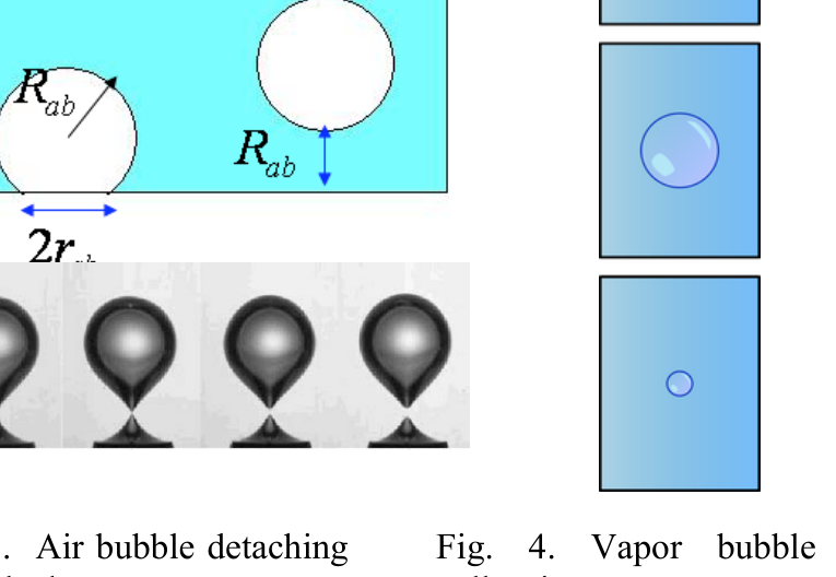Fig. 3. Air bubble detaching from the bottom.

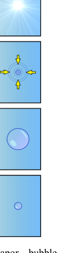Fig. 4. Vapor bubble collapsing.

Questions (total 10 points)

Consider water boiling in a flat-bottomed cylinder glass teakettle at normal atmospheric pressure. The bottom of the kettle heats up uniformly and a vertical temperature gradient exists, bubbles appear and evolve (Fig.2).

Q1. Write the pressure condition of the growth of an AB in the water volume at height h = H, when H is the water surface level in the kettle. Use the condition that the inside pressure must be greater than the outside one. Write down the inequality $2\pi r_{ab}>>P_{vapor}\pi r_{ab}^2$, [in terms of $P_a$, $P_v$, $R_{ab}$, $\rho$, $g$, $\sigma$, h, H] (1.0 point)

Q2. Write for an AB the wettability condition of the detachment from the bottom of the teakettle (Fig.3). Take into account the relation $r_{ab}<<R_{ab}$, [in terms of $r_{ab}$, $R_{ab}$, $\rho$, $\sigma$] (1.5 points)

Q3. Consider an AB with radius $R_a$ at the bottom of the teakettle. As water is boiled, the bubble is saturated with vapor and enlarges its radius. Write the ratio $\xi \equiv m_{air}/m_{vapor}$ of the masses of the air and saturated vapor inside the bubble at given temperature T. Calculate the ratio at room temperature T = 20 °C ($R_a=0.5$ mm) and at boiling point at T = 100 °C ($R_a=1$ mm). [in terms of ${\mu }_{air}$, T, $P_a$, $P_{vapor}$, $R_a$, $\rho$, ${\rho }_v$, $\sigma$, H] (1.5 points)

Q4. By using the NAE data and Newton’s Law estimate the radius of the AB detached from the bottom and uprised in distance $R_{ac}$ (Fig.3). Assume, that the added-mass (taking into account surrounding water layer) of AB is half of the analogous water bubble. (1.0 point)

Q5. Write the radius of the foundation of an AB just before the uprising, when the connecting “neck” is very narrow (see Fig.3). [in terms of $R_{ab}$, $\rho$, $\sigma$] Calculate it by using the radius found in Q4. (1.5 points)

Q6. By using the NAE data estimate the radius of collapsing VB (Fig.4) by assuming that the radial pressure is about 3kPa during this process. (1.2 points)

Q7. By using previous data for typical AB by using the Stokes law of a laminar flow. [in terms of $R_{ab}$, ${\rho }_w$, ${\eta }_w$] Estimate the uprising time for H = 10 cm. (0.6 points)

Q8. Write the apparent velocity for typical VB by using the Stokes law of a laminar flow. [in terms of $R_{ab}$, ${\rho }_w$, ${\eta }_w$] Estimate the uprising time for H = 10 cm. (1.2 points)

Q9. Write the average velocity of the elevation of VB with turbulent type of flow [in terms of $R_{ab}$, ${\rho }_w$, ${\eta }_w$] Estimate the uprising time for H = 10 cm. (1.2 points)

Fonte: Testo (PDF) — p.1

Topic: Fluid Mechanics, Thermodynamics Metodi: Hydrostatic Equilibrium, Ideal Gas Law, Order-of-Magnitude Estimation, Free-Body Diagram Competenze: Estimation & Approximation, Physical Reasoning Objects: Bubble, Container

Ceremonia del tè e fisica delle bolle

La cerimonia del tè è tradizionale in Asia. Uno degli importanti passi nella preparazione del tè è l’ebollizione dell’acqua dolce quando le bolle appaiono all’interno. Le bolle sono familiari dalla vita quotidiana e occupano un ruolo importante nella fisica, chimica, medicina e tecnologia. Tuttavia, il loro comportamento è spesso sorprendente e inaspettato e, in molti casi, ancora incomprensibile.

A temperatura ambiente l’acqua pura è satura di gas. Con l’aumento della temperatura, l’eccesso di pressione del gas sciolto $P_{gb}$ aumenta, l’aria sciolta viene liberata e le bolle d’aria (** ABs**) appaiono al fondo e alle pareti della cella di teacotta (Fig. 2). Per l’acqua pura la umidità è sufficiente e un AB rappresenta una sfera troncata con raggio $R_{ab}$ e con base non umida con raggio $r_{ab}<<R_{ab}$. Al caldo più elevato, le AB si espandono e raggiungendo determinate dimensioni possono distaccarsi dal fondo (Fig. 3), che si estende fino alla superficie dell’acqua e si scoppe lì. Le bolle di vapore (** VBs**) si presentano quando la temperatura dell’ acqua in fondo raggiunge il valore critico $T_{cr}^b=T_{cr0}^b=100{}^{\circ }C$ al quale la pressione del vapore saturo supera la pressione esterna. La produzione di vapore aumenta dieci volte, i VB si espandono e si staccano dal basso. Il VB può essere considerato costituito solo da vapore. Se l’acqua viene riscaldata abbastanza, la rivolta VB continua a gonfiarsi, raggiunge la superficie e esplode. Altrimenti, l’acqua non si riscalderà abbastanza negli strati superiori e uscirà da un forte gradiente di temperatura verticale. Per raggiungere livelli relativamente freddi di acqua, il VB crolla nel volume dell’acqua (Fig. 4). Ciò provoca la degasione indotta - forti oscillazioni e una notevole quantità di aria dissoluta viene rilasciata sotto forma di bolle d’aria microscopiche (** MAB**). Questo può generare vibrazioni a ultrasuoni.

Le principali fasi dell’evoluzione delle bolle durante il processo di ebollizione sono:

• l’aspetto e la crescita di AB al fondo e alle pareti, la loro trasmutazione in VB;
• il distacco e la rivolta del VB, la loro scomparsa nel volume dell’acqua o sulla superficie;
• l’apparenza di MAB nel volume dell’acqua e la loro ripresa in superficie.

Questa descrizione teorica è in buona accordo con gli esperimenti moderni. In particolare, è stato eseguito un interessante esperimento di analisi del rumore (NAE, Ural State University, Ekaterinburg) per l’acqua bollente. I microfoni altamente sensibili collegati ad amplificatori a banda larga e collegati a una cella elettrica hanno rilevato tre origini principali di rumore:

1. Distaccamenti di AB dal fondo prima di bollire (generizzare oscillazioni a ${\nu }_1\sim 100$ Hz);
2. I VB si riversano nel volume dell’acqua (generizzano oscillazioni con ${\nu }_2\sim 1$ kHz);
3. Le apparizioni di MAB sotto la superficie dell’acqua (generizzano oscillazioni da ${\nu }_3\sim 35$ kHz a 60 kHz).

Indizi

È noto che una piccola bolla si alza lungo un percorso rettilineare e si osserva un flusso laminare - l’acqua scorre facilmente e stratificatamente (vedere figura 1). Quindi, la formula di Stokes descrive la forza di dissipazione per una particella che si muove a bassa velocità $v_{slow}$: $F_d=6\pi {\eta }_w{R}_b{v}_{slow}$

In contrasto con questa immagine, quando le bolle relativamente grandi si alzano alla superficie, disturbano l’acqua circostante; dietro si trovano buche di cavitazione e si osserva il flusso turbolento (vedi Figura 1). In questo caso una parte dell’energia cinetica di una bolla di sollevamento si trasferisce nel lavoro di dissipazione.

Fig. 1. Tipo di flusso laminare e turbolento per le bolle d’aria in aumento nell’acqua.

Quando la superficie del liquido ha una forma convexa (concava) appare una forza di tensione superficiale dovuta all’interazione molecolare vicino al bordo. Questa pressione può quindi essere data con la formula $\Delta P=\frac{2\sigma }{R}$ se $\sigma$ è il coefficiente di tensione superficiale (unità = N/m), la forza che arriva all’unità di lunghezza della superficie, $R$ è il raggio di curvatura della superficie.

**3) ** Quando si tratta di un processo breve con durata caratteristica "$\tau$", il suo valore inverso può essere considerato come una frequenza caratteristica $\nu =\frac{1}{\tau }$. Utilizzare questa definizione per calcolare le frequenze del rumore.

Dati utili

• $P_a=1.016\cdot 10^5$ [Pa] - pressione atmosferica,
• ${\rho }_w=10^3$ [kg / m3] - densità dell’acqua,
• ${\rho }_{vapor}=0.017$ [kg / m3] - densità di vapore a T = 293 K; ($\zeta =0.596$ [kg / m3] a T = 373 K)
• $P_{vapor}=0.023\cdot 10^5$ [Pa] - pressione di vapore a T = 293 K; ($1.016\cdot 10^5$ [Pa] a T = 373 K)
• $g=9.81$ [m/s2] - accelerazione della gravità,
• ${\mu }_{air}=0.029$ [kg / mole] - peso molecolare dell’aria,
• $R=8.31$ [J / mole · K] - costante universale del gas,
• $\sigma =0.0725$ [N / m] - coefficiente di tensione superficiale dell’acqua,
• ${\eta }_w=0.3\cdot 10^{-3}$ [Pa · s] - coefficiente di viscosità dell’acqua,
• H = 10 cm Atteggiamento dell’acqua in teakettle.

Fig. 2. Bolle in teacettle.

Fig. 3. Bubble d’aria che si stacca dal fondo.

*Fig. 4. La bolla di vapore si sta crollando.

Domande (totalmente 10 punti)

Considera l’acqua che bolle in una cella di vetro a cilindro a fondo piatto a pressione atmosferica normale. Il fondo della caldaia si riscalda uniformemente e esiste un gradiente verticale di temperatura, le bolle appaiono ed evolvono (Fig.2).

Q1. Scrivere la condizione di pressione della crescita di un AB nel volume dell’acqua ad altezza h = H, quando H è il livello della superficie dell’acqua nel calciatore. Utilizzare la condizione che la pressione interna debba essere superiore a quella esterna. Scribire le disuguaglianze $2\pi r_{ab}>>P_{vapor}\pi r_{ab}^2$, [* in termini di $P_a$, $P_v$, $R_{ab}$, $\rho$, $g$, $\sigma$, h, H* (1.0 punto)

Q2. Scrivere per un AB la condizione di umidità del distacco dal fondo della cella di teacchetto (Fig.3). Si tiene conto della relazione $r_{ab}<<R_{ab}$, [* in termini di $r_{ab}$, $R_{ab}$, $\rho$, $\sigma$* (1,5 punti)

**Q3. ** Considerare un AB con raggio $R_a$ in fondo alla cucitura. Mentre l’acqua viene bollita, la bolla si satura di vapore e aumenta il suo raggio. Scrivere il rapporto $\xi \equiv m_{air}/m_{vapor}$ delle masse dell’aria e del vapore saturo all’interno della bolla a una determinata temperatura T. Calcolare il rapporto a temperatura ambiente T = 20 °C ($R_a=0.5$ mm) e al punto di ebollizione T = 100 °C ($R_a=1$ mm). [in termini di ${\mu }_{air}$, T, $P_a$, $P_{vapor}$, $R_a$, $\rho$, ${\rho }_v$, $\sigma$, H (1,5 punti)

Q4. Attraverso i dati NAE e la legge di Newton, si stima il raggio di AB distaccato dal fondo e sollevato a distanza $R_{ac}$ (Fig.3). Supponiamo che la massa aggiunta (tenendo conto dello strato di acqua circostante) di AB sia la metà della bolla d’acqua analogo. (1,0 punti)

Q5. Scrivi il raggio di fondazione di un AB poco prima dell’insurrezione, quando il “collo” di connessione è molto stretto (vedi figura 3). [* in termini di $R_{ab}$, $\rho$, $\sigma$ *] Calcolale utilizzando il raggio trovato in Q4. (1,5 punti)

Q6. Usando i dati NAE, si stima il raggio di VB in collasso (Fig.4) supponendo che la pressione radial sia di circa 3kPa durante questo processo. 1,2 punti)

Q7. Usando dati precedenti per un tipico AB, usando la legge di Stokes di un flusso laminare. [in termini di $R_{ab}$, ${\rho }_w$, ${\eta }_w$] Estimare il tempo di sollevazione per H = 10 cm. (0,6 punti)

**Q8. ** Scrivere la velocità apparente per VB tipico utilizzando la legge di Stokes di un flusso laminare. [in termini di $R_{ab}$, ${\rho }_w$, ${\eta }_w$] Estimare il tempo di sollevazione per H = 10 cm. 1,2 punti)

Q9. Scrivere la velocità media dell’altezza di VB con tipo turbolento di flusso [* in termini di $R_{ab}$, ${\rho }_w$, ${\eta }_w$*] Estimare il tempo di sollevazione per H = 10 cm. 1,2 punti)

Fonte: Testo (PDF) — p.1

Topic: Fluid Mechanics, Thermodynamics Metodi: Hydrostatic Equilibrium, Ideal Gas Law, Order-of-Magnitude Estimation, Free-Body Diagram Competenze: Estimation & Approximation, Physical Reasoning Objects: Bubble, Container

Ionic Crystal, Yukawa-type Potential and Pauli Principle

Atoms of many chemical elements possess very low ionization energy and easily lose the outer electrons. Vice versa, atoms of other elements accept easily the electrons. Taken into one volume, these positive and negative ions can combine into stable ionic structures. Many solids exhibit a crystal structure, in which the atoms are arranged in extremely regular, periodic patterns. In an ideal crystal the same basic structural unit is repeated through the space.

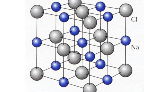Fig.1 — The face-centered cubic lattice of the sodium chloride (NaCl). The lattice spacing between the atomar centres is constant and is given by parameter $r_0$.

The main contribution to the binding energy of an ionic crystal is given by the electrostatic potential energy of ions.

The electric interaction acting between two point charges $q_1$ and $q_2$ standing in distance R is well defined by Coulomb’s potential: $V_C(R)=k\frac{q_1{q}_2}{R}$ where $k=1/4\pi {\epsilon }_0\approx 9\cdot 10^9$ [N · m² / C²] is the Coulomb constant. A negative force implies an attractive force. The force is directed along the line joining the two charges. For the case of NaCl crystals both types of ions has the unit charge $\pm e$ and one should also take into account many other neighbors acting on the chosen ion. Taking into account all positive and negative ions in a crystal of the infinite sizes results in the attractive potential energy $V_{att}(r)=\alpha \cdot V_C(r)$, where $r$ is the distance between nearest neighbors and $\alpha =1.74756$ is the Madelung constant [E. Madelung, Phys. Zs, 19 (1918) p542] and used in determining the energy of a single ion in a crystal.

Along the attractive potential energy there should to be a repulsive potential energy due to the Pauli Exclusion Principle and the overlap of electron shells in a crystal lattice. In contrast to the Coulomb-type attractive part, the repulsive potential energy is very short range.

There are two different models to describe the repulsive potential.

Model #1. A reasonable approximation to the repulsive potential is an exponential function: $V_{rep}(r)=\lambda \cdot e^{-r/\rho },(\lambda ,\rho >0)$ which describes the repulsion interaction of selected ion with the entire crystal lattice. Here $\lambda$ is coupling strength and $\rho$ stands for the range parameter.

Model #2. Another good approximation to the repulsive potential is an inverse power $V_{rep}(r)=b/r^n,(b>0)$ where $b$ is coupling strength and $n$ is integer greater than 1 (the Born exponent). These parameters take into account the repulsion with entire crystals.

Obviously, the physical parameters and model potentials depend on the type of crystal lattice.

Experimental data for the lattice constant $r_0$ and the dissociation energy $E_{\infty }$ (needed to break the lattice into separate ions) are given in Table 1 for some ionic crystals at normal temperature and pressure.

Table 1 — Properties of Salt Crystals with the NaCl Structure [C. Kittel, “Introduction to Solid State Physics”, N.Y., Wiley (1976) p.92] (in one mole there are the Avogadro’s number of pairs of ions or atoms).

Crystal	$r_0$ [nm]	$E_{\infty }$ [kJ / mole]
NaCl	0.282	−764.4
LiF	0.214	−1014.0
RbBr	0.345	−638.8

Questions (total 10 points)

Q1. Write down the Coulomb potential $V_{cr}(r)$ for an ion located at the centre of cubic lattice in Fig. 1. Let it interact only with the nearest neighbors (in distance up to and including $r=\sqrt{3}{r}_0$) of a crystal lattice. Find the Madelung constant ${\alpha }_c$ corresponding to this approximation. (1.5 points)

Q2. By using Model #1 write down the net potential energy per ion $V_1(r)$. Determine its equilibrium equation for $r=r_0$ and write down the net potential energy $V_1(r_0)$ [in terms of $\alpha ,r_0,\rho ,\lambda$]. Use exact Madelung constant $\alpha$. (1.5 points)

Q3. By using experimental data estimate the range parameter $\rho$. Use $N_A=6.022\cdot 10^{23}$ [1 / mole]. (2.0 points)

Q4. By using Model #2 write down the net potential energy $V_2(r)$ per ion. Determine its equilibrium position $r=r_0$ and write down the net potential energy $V_2(r_0)$. Use exact Madelung constant $n$. [in terms of $\alpha ,r_0,n$] (2.0 points)

Q5. By using experimental data (from Table 1) estimate the Born exponent $n$ for NaCl. Estimate the proportions of the Coulomb interaction and the Pauli exclusion (repulsive part) in the entire net potential energy in the equilibrium state? (1.5 points)

Q6. The ionization energy (required to extract an electron from an atom) of the Na atom is +5.14 eV, the electron affinity (required to receive an electron to an atom) of the Cl atom is −3.61 eV. Estimate the total binding energy (holds an atom inside lattice) per atom in the NaCl crystal. The experimental result is $E_{exp}=-3.28$ [eV]. [in terms of eV] Use the conversion that: 1 [eV] = $1.602\cdot 10^{-19}$ [J]. (1.5 points)

Fonte: Testo (PDF) — p.1

Topic: Electrostatics, Modern-Quantum Physics Metodi: Coulomb’s Law, Electric Potential Method, Energy Conservation Method, Superposition Principle Competenze: Mathematical Modeling, Physical Reasoning Objects: Point Charge, Atom

Cristallo ionico, potenziale di tipo Yukawa e principio di Pauli

Gli atomi di molti elementi chimici hanno una energia di ionizzazione molto bassa e perdono facilmente gli elettroni esterni. Al contrario, gli atomi di altri elementi accettano facilmente gli elettroni. Presi in un unico volume, questi ioni positivi e negativi possono combinarsi in strutture ioniche stabili. Molti solidi presentano una struttura cristallina, in cui gli atomi sono disposti in schemi periodici estremamente regolari. In un cristallo ideale la stessa unità strutturale di base si ripete attraverso lo spazio.

Fig.1 La rete cubica centrata sul viso del cloruro di sodio (NaCl). L’intervallo della rete tra i centri atomici è costante ed è dato dal parametro $r_0$.

Il contributo principale all’energia di legame di un cristallo ionico è dato dall’energia potenziale elettrostatica degli ioni.

L’interazione elettrica che agisce tra due cariche puntate $q_1$ e $q_2$ in posizione a distanza R è ben definita dal potenziale di Coulomb: $V_C(R)=k\frac{q_1{q}_2}{R}$ dove $k=1/4\pi {\epsilon }_0\approx 9\cdot 10^9$ [N · m2 / C2] è la costante di Coulomb. Una forza negativa implica una forza attraente. La forza è diretta lungo la linea che unisce le due cariche. Per i cristalli NaCl entrambi i tipi di ioni hanno la carica unitaria $\pm e$ e si dovrebbe anche tenere conto di molti altri vicini che agiscono sull’ion scelto. Tenendo conto di tutti gli ioni positivi e negativi in un cristallo di dimensioni infinite si ottiene l’energia potenziale **attraente ** $V_{att}(r)=\alpha \cdot V_C(r)$, dove $r$ è la distanza tra i vicini più vicini e $\alpha =1.74756$ è la costante Madelung [E. Madelung, fisico. Zs, 19 (1918) p542] e utilizzato per determinare l’energia di un singolo ione in un cristallo.

Lungo l’energia potenziale attraente dovrebbe esserci un’energia potenziale rifulsiva a causa del principio di esclusione di Pauli e della sovrapposizione di conchiglie elettroniche in una rete cristallina. A differenza della parte attraente del tipo Coulomb, l’energia potenziale repulsiva è di corto raggio.

Ci sono due modelli diversi per descrivere il potenziale repulsivo.

Modello #1. Un’approssimazione ragionevole del potenziale repulsivo è una funzione esponenziale: $V_{rep}(r)=\lambda \cdot e^{-r/\rho },(\lambda ,\rho >0)$ che descrive l’interazione di repulsione di uno di questi ioni con l’intera reticola di cristallo. Qui $\lambda$ è la forza di accoppiamento e $\rho$ rappresenta il parametro di gamma.

Modello #2. Un’altra buona approssimazione del potenziale repulsivo è una potenza inversa $V_{rep}(r)=b/r^n,(b>0)$ dove $b$ è la forza di accoppiamento e $n$ è un numero intero superiore a 1 (esponente Born). Questi parametri tengono conto della repulsione con cristalli interi.

Ovviamente, i parametri fisici e i potenziali del modello dipendono dal tipo di reticola di cristallo.

I dati sperimentali per la costante della reticola $r_0$ e l’energia di dissociazione $E_{\infty }$ (necessaria per spezzare la reticola in ioni separati) sono riportati nella tabella 1 per alcuni cristalli ionici a temperatura e pressione normali.

Tabella 1 Proprietà dei cristalli di sale con struttura NaCl [C. Kittel, “Introduzione alla fisica dello stato solido”, N.Y., Wiley (1976) p.92] (in un mole ci sono i numeri di ioni o atomi di Avogadro).

Crystal	$r_0$ [nm]	$E_{\infty }$ [kJ / mole]

NaCl # 0.282 - 764.4

# La vita # # 0.214 # -1014.0

# RbBr # 0.345 # -638.8

Domande (totalmente 10 punti)

Q1. Scrivi il potenziale di Coulomb $V_{cr}(r)$ per un ione situato al centro della reticola cubica nella figura. 1. Lasciate che interagisca solo con i vicini più vicini (a distanza fino a $r=\sqrt{3}{r}_0$) di una griglia cristallina. Trova la costante Madelung ${\alpha }_c$ corrispondente a questa approssimazione. (1,5 punti)

Q2. Con il modello #1, calcolare l’energia potenziale netta per ione $V_1(r)$. Determinare la sua equazione di equilibrio per $r=r_0$ e annotare l’energia potenziale netta $V_1(r_0)$ [* in termini di $\alpha ,r_0,\rho ,\lambda$*. Utilizzare la costante Madelung esatta $\alpha$. (1,5 punti)

Q3. Attraverso dati sperimentali, calcolare il parametro di gamma $\rho$. Utilizzare $N_A=6.022\cdot 10^{23}$ [1 / mole]. (2,0 punti)

Q4. Con il modello #2 si registra l’energia potenziale netta $V_2(r)$ per ione. Determinare la sua posizione di equilibrio $r=r_0$ e annotare l’energia potenziale netta $V_2(r_0)$. Utilizzare la costante Madelung esatta $n$. [* in termini di $\alpha ,r_0,n$*] (2,0 punti)

**Q5. ** Attraverso dati sperimentali (da cui figura la tabella 1) si stima l’ esponente Born $n$ per NaCl. Estimare le proporzioni dell’interazione di Coulomb e dell’esclusione di Pauli (parte repulsiva) nell’intera energia potenziale netta nello stato di equilibrio? (1,5 punti)

Q6. L’energia di ionizzazione (requisita per estrarre un elettrone da un atomo) dell’atomo Na è +5.14 eV, l’affinità elettronica (requisita per ricevere un elettrone ad un atomo) dell’atomo Cl è −3.61 eV. Calcolare l’energia di legame totale (che contiene un atomo all’interno della griglia) per atomo nel cristallo NaCl. Il risultato sperimentale è $E_{exp}=-3.28$ [eV]. [in termini di eV] Utilizzare la conversione che: 1 [eV] = $1.602\cdot 10^{-19}$ [J]. (1,5 punti)

Fonte: Testo (PDF) — p.1

Topic: Electrostatics, Modern-Quantum Physics Metodi: Coulomb’s Law, Electric Potential Method, Energy Conservation Method, Superposition Principle Competenze: Mathematical Modeling, Physical Reasoning Objects: Point Charge, Atom

How does a superluminal object look like?

Can a body move faster than the speed of light? The answer is “No” if the object is moving in the vacuum. But the answer can be “Yes”, if we deal with the phase speed of light in an optically dense medium with refractive index of $n$ ($n=c/u$, where $u$ is the speed of light in the medium, and $c$ is the speed of light in the vacuum).

We say a body is superluminal, if $u<v<c$, where $v$ is the velocity of the body. One of the well known examples of the superluminal body is a charged particle generating Cherenkov radiation.

Throughout the problem we will deal with a superluminal body of constant velocity $v$ in an optical medium without dispersion. $u$ is the velocity of light in the medium.

For the simplicity, we introduce a notation $\gamma =\frac{1}{\sqrt{1-(v/c{)}^2}}$ and an angle $\theta$ given by $\cos \theta =u/v$ and $\tan \theta =\sqrt{\frac{v^2}{u^2}-1}$.

1. Radiating superluminal particle

As shown in Fig.1, a radiating particle is moving along the $x$-axis with a constant velocity $v$ ($v>u$).

An observer $M$ is located at the distance $d$ from $x$-axis.

We choose the point nearest to the observer as the point $O$, the origin on the $x$-axis. The time when the particle actually passes over the point $x=0$ is taken to be $t=0$.

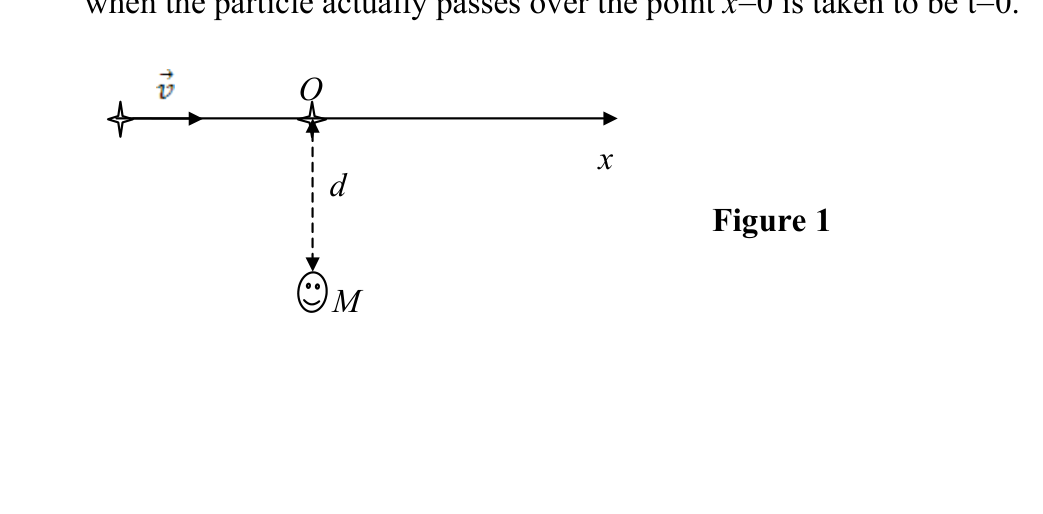Figure 1

(1) Suppose the light radiated at the given time $t^{\prime }$ is observed at time $t$. Express $t$ in terms of $d,t^{\prime },u$ and $v$. (1.0 point)

(2) At time $t=t_0$, the observer first sees the particle at position $x_0^{\prime }$. Find the apparent position $x_0^{\prime }$ and the observed time $t_0$ for this first appearance in terms of $d,v$ and $\theta$. (2.0 points)

(3) Find the apparent position(s) $x^{\prime }$ of the particle for any given time $t$. Write your answer in terms of $v,\theta ,t$ and $t_0$. (2.0 points)

(4) Find the apparent velocity(s) $v^{\prime }(t)$ of the particle for any given time $t$. Write your answer in terms of $v,\theta ,t$, and $t_0$. (1.0 point)

(5) Find the apparent velocity(s) $v^{\prime }$ of the first appearance of the particle. (0.2 points)

(6) Find the apparent velocity(s) $v^{\prime }$ of the particle at infinite distances from the origin, $O$. Write your answer in terms of $v$ and $u$. (0.2 points)

(7) Sketch the graph of the apparent velocity $v^{\prime }$ versus time $t$, indicating clearly asymptotic values of the apparent velocity. (1.0 point)

(8) Can an apparent velocity exceed the light speed in the vacuum, i.e. $v^{\prime }>c$? (0.2 points)

2. Radiating linear object

Consider a linear object, radiating light and moving along the $x$-axis. The length of the linear object is $L$ in the rest frame of the object.

A. Parallel movement

In this section, we assume that the radiating linear object moves longitudinally along $x$-axis as shown in Fig.2.

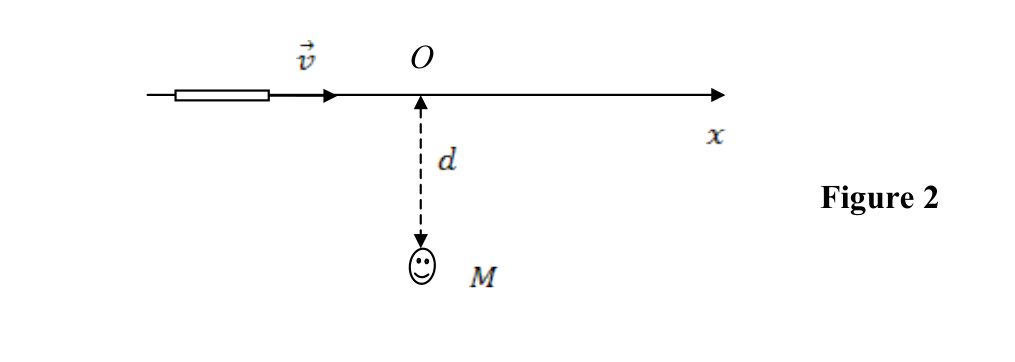Figure 2

(9) Determine the time interval of complete appearance of the whole linear object from the first appearance of its front point. Write your answer in terms of $L,\gamma$ and $v$. (0.3 points)

(10) Determine the apparent length(s) of the object at the moment of its complete appearance. Write your answer in terms of $d,L,\theta$ and $\gamma$. (0.4 points)

B. Perpendicular movement

In this section, we assume that the radiating linear object moves perpendicularly along $x$-axis as shown in Fig.3. Let the observer be located at the origin of $x$-axis ($d=0$). The object is symmetrical with respect to $x$-axis.

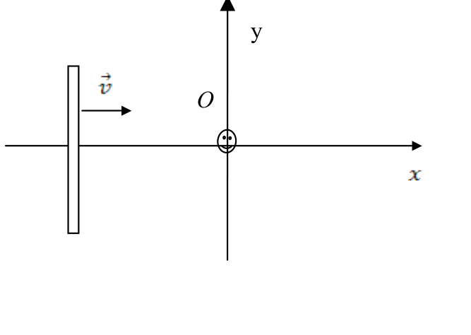Figure 3

(11) Show that for a given time $t$, the apparent form of this object is an ellipse or part(s) of an ellipse. (0.7 points)

Find the following quantities and express them in terms of $v,\theta$, and $t$.

(12) Find the position $x_c$ of the centre of symmetry of the ellipse for a given time $t$ in terms of $v,\theta$ and $t$. (0.5 points)

(13) Determine the lengths of the semi-major and semi-minor axes of the ellipse for a given time $t$ in terms of $v,\theta$ and $t$. (0.5 points)

Fonte: Testo (PDF) — p.1

Topic: Special Relativity, Geometric Optics Metodi: Lorentz Transformation, Kinematic Equations, Vector Decomposition, Approximation & Series Expansion Competenze: Mathematical Modeling, Diagrammatic Reasoning Objects: Point Charge

Come è un oggetto superluminale?

Un corpo può muoversi più velocemente della luce? La risposta è “No” se l’oggetto si muove nel vuoto. Ma la risposta può essere “Sì”, se si tratta della velocità di fase della luce in un mezzo otticamente denso con un indice di rifrazione di $n$ ($n=c/u$, dove $u$ è la velocità della luce nel mezzo, e $c$ è la velocità della luce nel vuoto).

Diciamo che un corpo è superluminale, se $u<v<c$, dove $v$ è la velocità del corpo. Uno degli esempi ben noti del corpo superluminale è una particella carica che genera radiazioni di Cherenkov.

Durante tutto il problema si tratta di un corpo superluminario di velocità costante $v$ in un mezzo ottico senza dispersione. $u$ è la velocità della luce nel mezzo.

Per semplicità, introduciamo una notazione $\gamma =\frac{1}{\sqrt{1-(v/c{)}^2}}$ e un angolo $\theta$ dato da $\cos \theta =u/v$ e $\tan \theta =\sqrt{\frac{v^2}{u^2}-1}$.

1. Particelle superluminali irradianti

Come mostrato nella figura 1, una particella irradiante si muove lungo l’asse $x$ con una velocità costante $v$ ($v>u$).

Un osservatore $M$ si trova alla distanza $d$ dall’asse $x$.

Scegliamo il punto più vicino all’osservatore come punto $O$, l’origine sull’asse $x$. Il tempo in cui la particella effettivamente passa sopra il punto $x=0$ è considerato $t=0$.

Figura 1

**(1) ** Supponiamo che la luce irradiata al momento dato $t^{\prime }$ sia osservata al momento $t$. Esprimere $t$ in termini di $d,t^{\prime },u$ e $v$. (1,0 punti)

**(2) ** Al tempo $t=t_0$, l’osservatore vede per la prima volta la particella in posizione $x_0^{\prime }$. Trova la posizione apparente $x_0^{\prime }$ e il tempo osservato $t_0$ per questa prima comparsa in termini di $d,v$ e $\theta$. (2,0 punti)

**(3) ** Trova la posizione apparente delle particelle $x^{\prime }$ per un dato tempo $t$. Scrivi la tua risposta in termini di $v,\theta ,t$ e $t_0$. (2,0 punti)

**(4) ** Trova la velocità apparente (s) $v^{\prime }(t)$ della particella per un dato tempo $t$. Scrivi la tua risposta in termini di $v,\theta ,t$ e $t_0$. (1,0 punti)

**(5) ** Trova la velocità apparente (s) $v^{\prime }$ della prima comparsa della particella. (0,2 punti)

**(6) ** Trova la velocità apparente (s) $v^{\prime }$ della particella a distanze infinite dall’origine, $O$. Scrivi la tua risposta in termini di $v$ e $u$. (0,2 punti)

**(7) ** Segnare il grafico della velocità apparente $v^{\prime }$ contro il tempo $t$, indicando chiaramente i valori asimptotici della velocità apparente. (1,0 punti)

**(8) ** Una velocità apparente può superare la velocità della luce nel vuoto, ovvero $v^{\prime }>c$? (0,2 punti)

2. Obbiettivo lineare irradiante

Considera un oggetto lineare che irradia luce e si muove lungo l’asse $x$. La lunghezza dell’oggetto lineare è $L$ nel quadro del resto dell’oggetto.

A. Movimento parallelo

In questa sezione, supponiamo che l’oggetto lineare radiante si muova longitudinalmente lungo l’asse $x$ come mostrato nella figura 2.

Figura 2

**(9) ** Determinare l’intervallo temporale di apparenza completa dell’intero oggetto lineare dalla prima apparenza del suo punto di fronte. Scrivi la tua risposta in termini di $L,\gamma$ e $v$. (0,3 punti)

**(10) ** Determina la lunghezza apparente dell’oggetto al momento della sua completa comparsa. Scrivi la tua risposta in termini di $d,L,\theta$ e $\gamma$. (0,4 punti)

B. Movimento perpendicolare

In questa sezione, supponiamo che l’oggetto lineare radiante si muova perpendicolare lungo l’asse $x$ come mostrato in Figura 3. L’osservatore deve essere situato all’origine dell’asse $x$ ($d=0$). L’oggetto è simmetrico rispetto all’asse $x$.

Figura 3

**(11) ** Mostra che per un dato tempo $t$, la forma apparente di questo oggetto è un’ellisse o parti di un’ellisse. (0,7 punti)

Trova le seguenti quantità e esprimele in termini di $v,\theta$ e $t$.

**(12) ** Trova la posizione $x_c$ del centro di simmetria dell’ellisse per un dato tempo $t$ in termini di $v,\theta$ e $t$. (0,5 punti)

**(13) ** Determinare le lunghezze degli assi semi-maggiori e semi-minori dell’ellisse per un determinato tempo $t$ in termini di $v,\theta$ e $t$. (0,5 punti)

Fonte: Testo (PDF) — p.1

Topic: Special Relativity, Geometric Optics Metodi: Lorentz Transformation, Kinematic Equations, Vector Decomposition, Approximation & Series Expansion Competenze: Mathematical Modeling, Diagrammatic Reasoning Objects: Point Charge