APhO 2010 — Sperimentale

Experimental components

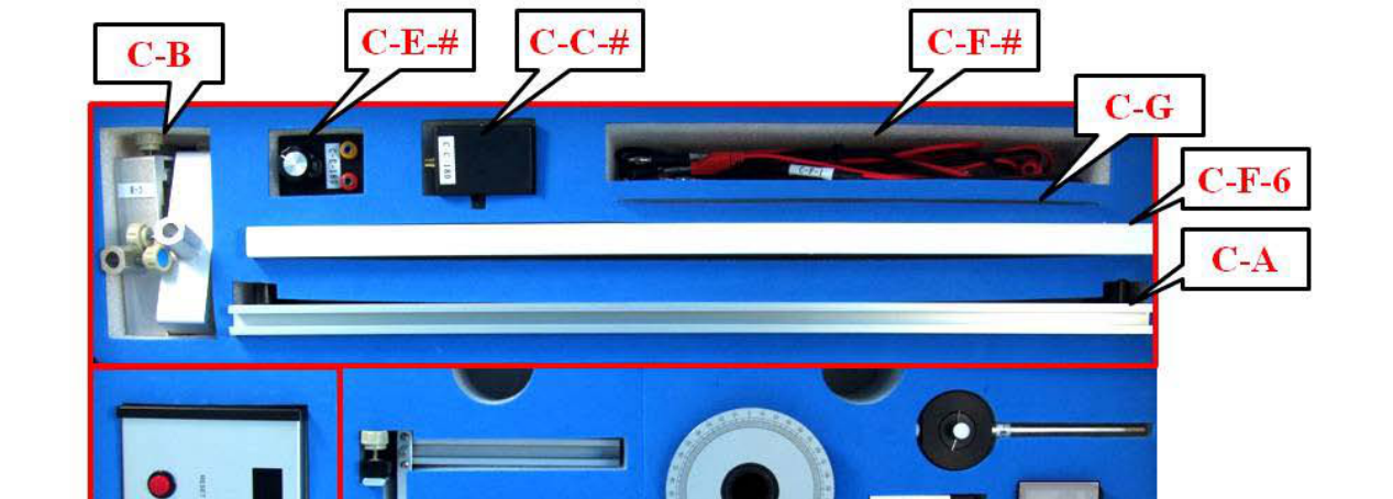
Set-C for common components:

Label	Items	Quantity
C-A	Optical track (60 cm)	1
C-B	Optical clamps	4
C-C-#	Collimated laser diode (CLD)	1
C-D-#	Sine wave generator (sine wave, DC 5V output)	1
C-E-#	Variable resistor ($5\text{k}\Omega$)	1
C-F-#	Connecting wires	4
C-F-6	Component stand	1
C-G	Ruler	1

Note: ”#” is the serial number for the component. This number is for examiner’s use.

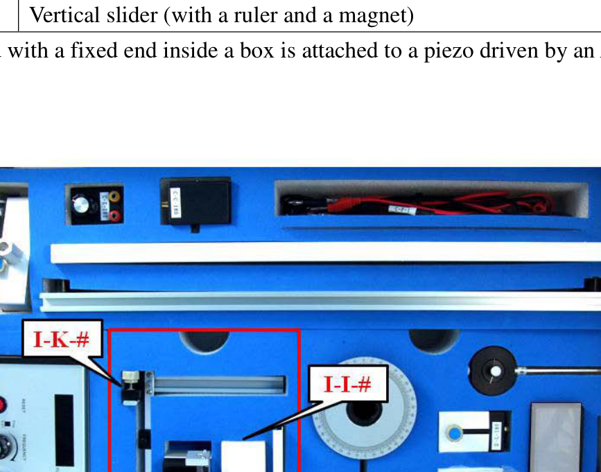
Set-I for Experiment-I:

Label	Items	Quantity
I-H-#	Black box on a 1-D translational stage	1
I-I-#	Brass reed attached to a driving box*	1
I-J	Screen for amplitude measurement	1
I-K-#	Vertical slider (with a ruler and a magnet)	1

*The brass reed with a fixed end inside a box is attached to a piezo driven by an AC voltage.

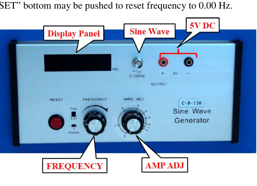
Instructions for the Sine Wave Generator:

• The power button, not shown in the picture, is on the right-hand side of the instrument.
• The “Display Panel” shows the frequency of the output sine wave.
• Use the “Sine Wave” BNC connector for supplying a sine wave voltage.
• Use the “5V DC” banana connectors for supplying a constant voltage of 5V.
• The frequency of the sine wave can be changed by turning the “FREQUENCY” knob, faster for coarse adjustment and slower for fine adjustment. Ignore the fine and coarse labels next to the “FREQUENCY” knob.
• The amplitude of the sine wave voltage can be adjusted by turning the “AMPL ADJ” knob.
• The “RESET” button may be pushed to reset frequency to 0.00 Hz.

Set-II for Experiment-II:

Label	Items	Quantity
II-L-#	Uncollimated laser diode (ULD)	1
II-M	Holders for ULD	1
II-P-#	Polarizer with indicator (PR2)	1
II-Q-#	Polarizer (PR1)	1
II-R	Holder for PR1 and PR2	1
II-T	Holder for light filter	1
II-U	Light filters	4
II-V	Beam viewing box (screen)	1
II-W-#	Photoconductor (PC)	1
II-X	Digital multimeter	1
II-Y	Digital multimeter	1

Items II-L-#, II-M, and II-V are not used.

Instructions for the digital multimeter:

• You can turn the digital multimeter on or off by pressing the power button.
• Use the “V$\Omega$” and the “COM” inlets for voltage and resistance measurements.
• Use the “mA” and the “COM” inlets for small current measurements.
• Use the function dial to select the proper function and measuring range. “V” is for voltage measurement, “A” is for current measurement and "$\Omega$" is for resistance measurement.
• Do not press the “HOLD” button, which will hold the display reading and stop the measurement function. You can release it by pressing the button again.

Experiment I. Magnetic force probe

Introduction

As shown in Fig. I-1, the free end of a reed can oscillate in the vertical direction when it is driven by an external oscillating force, and its frequency is determined by the external driver. If we plot the average power dissipated in the vibrating reed, which has certain damping mechanisms, as a function of frequency, we can find a maximum dissipated power at a certain frequency called the resonance frequency $f_R$, as illustrated in Fig. I-2. The sharpness of the resonance is described by the quality factor $Q$ as:

$Q=\frac{f_R}{\Delta f}$

where $\Delta f$ is the full width at half maximum of the $P_{av}$–$f$ curve, as shown in Fig. I-2, i.e. $\Delta f=f_2-f_1$ with $f_1$ and $f_2$ corresponding to $\frac{P_{max}}{2}$ on the lower side and the higher side of the resonance frequency respectively.

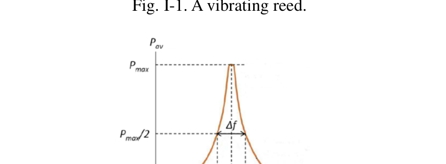
Fig. I-1. A vibrating reed.

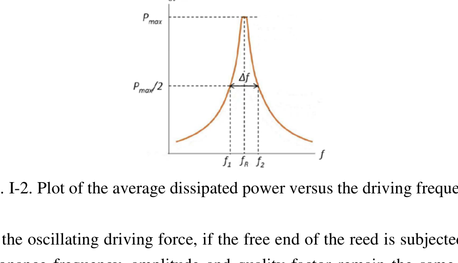
Fig. I-2. Plot of the average dissipated power versus the driving frequency.

Besides the oscillating driving force, if the free end of the reed is subjected to a uniform force, its resonance frequency, amplitude and quality factor remain the same. On the other hand, under a non-uniform force, many properties of the vibrating reed, such as the resonance frequency $f_R$, the maximum amplitude $A$, and the quality factor $Q$, may vary with the position of its free end.

In this experiment, a small magnet adhered to the free end of the reed serves as a probe tip as shown in Fig. I-3, while a target magnet underneath the tip magnet produces a non-uniform magnetic field and exerts a non-uniform force on the tip magnet. When the tip magnet approaches the target magnet underneath with same pole opposing each other, then the repulsive force becomes stronger. Thus the resonance frequency $f_R$ of the reed varies with the distance between the tip magnet and the target magnet. The resonance frequency increases with decreasing separation distance between the two repulsing magnets. However, when moving the tip magnet horizontally away from the target magnet as shown in Fig. I-4, it may sense a weak attractive force at a certain distance. The resonance frequency shifts to lower values when the non-uniform force is attractive. We shall use this property, that the resonance frequency of the reed sensitively depends on the separation between the tip magnet and target magnet, to locate the hidden magnets inside a black box.

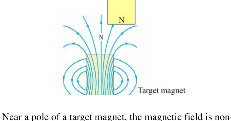
Fig. I-3. Near a pole of a target magnet, the magnetic field is non-uniform.

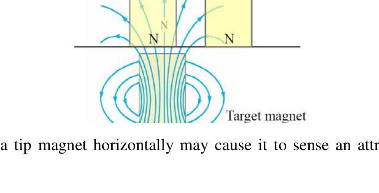
Fig. I-4. Moving a tip magnet horizontally may cause it to sense an attractive or repulsive force.

Experimental procedures

Error analysis is not required in any parts of Experiment I.

Exp. I-A. Measuring the resonance frequency

Carefully take out the experimental components from Set-C and Set-I, and set up the experimental apparatus as shown in Fig. I-A-1. The schematic plot is shown in Fig. I-A-2. Connect the 5V-DC voltage source to the laser box (C-C-#). Connect the oscillating output of the sine wave generator to the driving box of the brass reed (I-I-#). Turn on the power and fix the output voltage of the sine wave generator. Direct the laser beam into the mirror at the free end of the brass reed so that the reflected beam spot on the screen (I-J) can be used to determine the vibrating amplitude of the reed.

Caution:

1. Carefully remove the paper protected cover before using the brass reed (I-I-#) for experimental measurements. The resonance frequency of the brass reed is very sensitive to its shape, and any deformation of reed during the experiment may give an inaccurate result.
2. Do not directly look into the laser beam, which can damage your eyes.

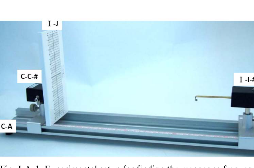
Fig. I-A-1. Experimental setup for finding the resonance frequency.

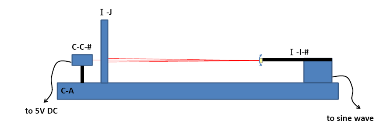
Fig. I-A-2. The schematic plot of Fig. I-A-1.

(1) Measure the amplitude $A$ of the oscillating laser beam spot by changing the frequency of the sine wave generator. Record the measured amplitude as a function of frequency in the data table on the answer sheet. (0.8 points)

(2) Make a proper plot on one of the supplied graph papers to determine the resonance frequency $f_{RO}$ and quality factor $Q$. Also record the obtained $f_{RO}$ and $Q$ in the proper blank spaces on the answer sheet. (1.2 points)

Exp. I-B. Resonance frequency versus the external force

In this part of experiment, the resonance frequency under the influence of a non-uniform force is investigated. The non-uniform force is provided by a small 3-mm cylindrical metallic calibration magnet $M_C$ fixed on a vertical slider (I-K-#) with its N pole pointing upward. The tip magnet $M_T$, adhered at the free end of the oscillating reed, has its N pole pointing downward. The pole axes of both magnets should be aligned along the same vertical line.

Set up the experiment as shown in Fig. I-B-1. The schematic plot is shown in Fig. I-B-2.

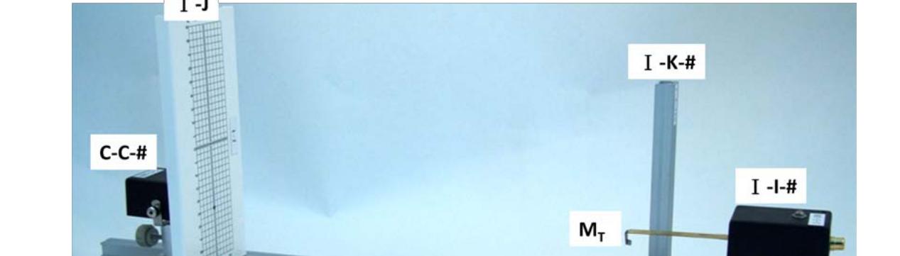
Fig. I-B-1. Experimental setup of finding the relation of resonance frequency with the nominal distance between two magnets, $M_C$ and $M_T$.

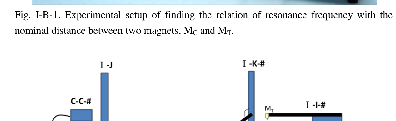
Fig. I-B-2. The schematic plot of Fig. I-B-1.

(1) On the scale of the vertical slider, read out the position $z_0$ of the bottom plane for the tip magnet $M_T$ without the interaction of $M_C$ by properly moving $M_C$ away from $M_T$. Record the measured $z_0$ in the data table. (0.2 points)

(2) Adjust the position of the magnet $M_C$ to be right underneath $M_T$. The pole axes of both magnets should be aligned along the same vertical line. Determine the position $z$ of the top plane of the N-pole of $M_C$. Calculate the nominal distance $d$ by defining $d=z_0-z$. Record $z$ and $d$ in the data table. (Note: The equilibrium separation between the two magnets is not the same as $d$ because the two magnets repel each other.)

(3) Determine the resonance frequency $f_R$ for the distance $d$ by tuning the frequency of the sine wave generator until the maximum amplitude is reached, plotting amplitude versus frequency is not necessary for determining $f_R$ of each distance $d$. Record the determined resonance frequency $f_R$ in the data table.

(4) Change the vertical position of the magnet $M_C$ and repeat the steps (2) and (3) for a number of measurements of different distance $d$ and the corresponding resonance frequency $f_R$. (1.2 points)

(5) Plot a graph of $f_R$ as a function of distance $d$ using a graph paper. Guiding by eyes, draw the best line through the data points. (1.2 points)

(6) Define $\Delta f_R=f_R-f_{RO}$, and plot $\ln (\Delta f_R)$ as a function of $d$ using another graph paper. Guiding by eyes, draw the best line through the data points. (1.0 points)

Exp. I-C. Finding the positions and depths of the magnets inside a black box

There are two magnets $M_A$ and $M_B$ buried in the black box (I-H-#) which is fixed on a 1D translational stage. The N poles of both magnets are pointed upward. Magnets $M_A$ and $M_B$, and $M_C$ used in Exp. I-B are very close in size, shape, and magnetic properties. The depths of the magnets $M_A$ and $M_B$ may be different. Magnet $M_A$ is located at the intersection of the two lines marked on the top surface of the black box. Magnet $M_B$ is located somewhere along the longer line as shown in Fig. I-C-1. The horizontal distance between magnets $M_A$ and $M_B$ is denoted by $\overline{AB}$.

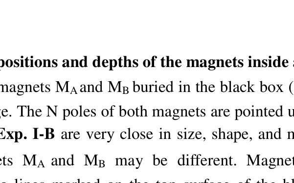
Fig. I-C-1. Magnet $M_A$ is located beneath the intersection of the two lines marked on the top surface while the magnet $M_B$ is located somewhere along the longer line.

(1) On the scale of the vertical slider, read out the position $z_0$ (in this part, $z_0$ may be different from the $z_0$ in Exp. I-B) of the bottom plane for the tip magnet $M_T$ without the interaction of the magnets inside the black box. On the scale of the vertical slider, read out the position $z_{box}$ of the top plane of black box. Record $z_0$ and $z_{box}$ on the answer sheet. (0.2 points)

(2) Move the black box along the longer line and observe the variation in resonance frequency $f_R$ of the reed to find the position of $M_B$. Record the measured distances $y$ and their corresponding resonance frequencies $f_R$ in the data table. (1.4 points)

(3) Plot $f_R$ as a function of $y$ on a graph paper to determine the position of magnet $M_B$. Mark the positions of magnets $M_A$ and $M_B$ on the $y$-axis of your graph, and write down the value of $\overline{AB}$ on the answer sheet. (1.2 points)

(4) Determine the depths $d_A$ and $d_B$ of the magnets $M_A$ and $M_B$ from the top surface of the black box using the results in Exp. I-B. Write down the values of $d_A$ and $d_B$ on the answer sheet. (1.6 points)

Fonte: Testo (PDF) — p.1 Topic: Oscillations & Waves, Magnetism Metodi: Experimental Data Analysis, Simple Harmonic Motion Analysis, Graph Linearization, Physical Modeling Competenze: Experimental Data Analysis, Measurement & Instrumentation, Graph Linearization, Physical Reasoning Objects: Magnet, Mirror

Componenti sperimentali

**Sett-C per componenti comuni: **

etichettare gli articoli quantità |---|---|---| ♬ C-A ♬ Track ottico 60 cm ♬ 1

C-B # Clamps ottiche

➡️C-C-# Diodo laser collimato ➡️ ♬ C-D-# ♬ Generatore d’onda sinistra | C-E-# | Variable resistor ($5\text{k}\Omega$) | 1 | ♬ C-F-# Collegare i fili ♬ 4 ♬ ♬ C-F-6 ♬ Componente stand ♬ 1 ♬ ♬ C-G ♬ Regola ♬ 1 ♬

Nota: ”#” è il numero di serie del componente. Questo numero è per l’uso dell’esaminatore.

**Sett-I per l’esperimento-I: **

etichettare gli articoli quantità |---|---|---| ♬ I-H-# ♬ Black box su una traduzione in 1D ♬ | I-I-# | Brass reed attached to a driving box* | 1 | ♬ I-J ♬ schermo per la misurazione dell’ampiezza ♬ 1 ♬ I-K-# ♬ Slider verticale (con una regola e un magnete) ♬ 1 ♬

*The brass reed with a fixed end inside a box is attached to a piezo driven by an AC voltage.

**Instruzioni per il generatore di onde sinologiche: **

• Il pulsante di alimentazione, non mostrato nella foto, è sul lato destro dello strumento.
• Il “Panel di visualizzazione” mostra la frequenza dell’onda sinusa di uscita.
• Usa il connettore BNC “Sine Wave” per fornire una tensione sinusa.
• Utilizzare i connettori banani “5 V DC” per fornire una tensione costante di 5 V.
• La frequenza dell’onda sinusa può essere modificata girando il pulsante “FREQUENCY”, più veloce per l’aggiustamento grosso e più lento per l’aggiustamento fine. Ignora le etichette fine e grossolane accanto al pulsante “FREQUENCY”.
• L’ampiezza della tensione sinusale può essere regolata girando il pulsante “AMPL ADJ”.
• Il pulsante ” RISET ” può essere premuto per resettare la frequenza a 0,00 Hz.

**Sett II per l’esperimento-II: **

etichettare gli articoli quantità |---|---|---| ♬ II-L-# Uncollimated laser diode (ULD) ♬ 1 ♬ ♬ II-M ♬ Tenitori per ULD ♬ 1 ♬ II-P-# ♬ Polarizzatore con indicatore ♬ ♬ II-Q-# Polarizzatore (PR1) ♬ 1 ♬ ➡️ II-R ➡️ Tenere per PR1 e PR2 ➡️ 1 ♬ Il filtro di luce ♬ ♬ II-U ♬ Filtri leggeri ♬ 4 ♬ ♬ II-V ♬ Scattoli di visualizzazione del fascio ♬ 1 ♬ ♬ II-W-# Fotoconduttore (PC) ♬ 1 ♬ ∙ 2X ∙ Multimetro digitale ∙ 1 ♬ II-Y ♬ Multimetro digitale ♬ 1

Non sono utilizzati i punti II-L-#, II-M e II-V.

Instruzioni per il multimetro digitale:

• Puoi accendere o spegnere il multimetro digitale premendo il pulsante di alimentazione.
• Per le misure di tensione e resistenza utilizzare le entrate “V$\Omega$” e “COM”.
• Utilizzare le entrate “mA” e “COM” per le piccole misurazioni di corrente.
• Utilizzare il quadrante di funzione per selezionare la funzione e la gamma di misura adeguate. “V” è per la misura della tensione, “A” è per la misura della corrente e "$\Omega$" è per la misura della resistenza.
• Non premere il pulsante “RITERARE”, che fermerà la lettura del display e fermerà la funzione di misurazione. Puoi rilasciarlo premendo di nuovo il pulsante.

L’esperimento I. Sonda di forza magnetica

**Introduzione **

Come mostrato nella figura. I-1, l’estremità libera di una canna può oscillarsi in direzione verticale quando è guidata da una forza oscillante esterna, e la sua frequenza è determinata dal conducente esterno. Se tracciamo la potenza media dissipata nella canna vibratrice, che ha determinati meccanismi di attenuazione, come funzione di frequenza, possiamo trovare una potenza massima dissipata a una certa frequenza chiamata frequenza di risonanza $f_R$, come illustrato nella figura. I-2. La nitidezza della risonanza è descritta dal fattore di qualità $Q$ come:

$Q=\frac{f_R}{\Delta f}$

dove $\Delta f$ è la larghezza completa alla metà massima della curva P_{av}$$f, come mostrato nella figura. I-2, i.e. $\Delta f=f_2-f_1$ con $f_1$ e $f_2$ corrispondenti a $\frac{P_{max}}{2}$ sul lato inferiore e sul lato superiore della frequenza di risonanza rispettivamente.

• Non è vero. I-1. Una canna vibrante.](../_attaccamenti/APhO_2010_exp/APhO_2010_exp_Q1_p6_f1.png)

Fig. - Cosa? I-1. Una canna vibrante.

• Non è vero. I-2. Indice della potenza media dissipata rispetto alla frequenza di guida.](../_attaccamenti/APhO_2010_exp/APhO_2010_exp_Q1_p6_f2.png)

Fig. - Cosa? I-2. Tracciato della potenza media dissipata rispetto alla frequenza di guida.

Oltre alla forza motrice oscillante, se l’estremità libera della canna è sottoposta a una forza uniforme, la frequenza di risonanza, l’ampiezza e il fattore di qualità rimangono gli stessi. D’altra parte, sotto una forza non uniforme, molte proprietà della canna vibrante, come la frequenza di risonanza $f_R$, l’ampiezza massima $A$ e il fattore di qualità $Q$, possono variare con la posizione della sua estremità libera.

In questo esperimento, un piccolo magnete aderito all’estremità libera della canna serve come punta di sonda come mostrato in Figura. I-3, mentre un magnete bersaglio sotto il magnete di punta produce un campo magnetico non uniforme ed esercita una forza non uniforme sul magnete di punta. Quando la punta di magnete si avvicina al magnete bersaglio sotto con lo stesso polo opposto l’uno all’altro, allora la forza repulsiva diventa più forte. La frequenza di risonanza $f_R$ della canna varia quindi con la distanza tra il magnete di punta e il magnete di destinazione. La frequenza di risonanza aumenta con la diminuzione della distanza di separazione tra i due magneti respingenti. Tuttavia, quando si sposta orizzontalmente il magnete di punta dal magnete di destinazione come mostrato nella figura. I-4, potrebbe percepire una debole forza di attrazione a una certa distanza. La frequenza di risonanza si sposta a valori inferiori quando la forza non uniforme è attraente. Utilizziamo questa proprietà, che la frequenza di risonanza della canna dipende sensibilmente dalla separazione tra il magnete di punta e il magnete di obiettivo, per individuare i magneti nascosti all’interno di una scatola nera.

• Non è vero. I-3. In prossimità di un polo di un magnete obiettivo, il campo magnetico non è uniforme.](../_attaccamenti/APhO_2010_exp/APhO_2010_exp_Q1_p7_f1.png)

Fig. - Cosa? I-3. Vicino a un polo di un magnete obiettivo, il campo magnetico non è uniforme.

• Non è vero. I-4. Movere un magnete a punta orizzontale può causare la percezione di una forza attraente o repulsiva.](../_attaccamenti/APhO_2010_exp/APhO_2010_exp_Q1_p7_f2.png)

Fig. - Cosa? I-4. Movere un magnete orizzontale può far sì che percepisca una forza di attrazione o di respiro.

Procedimenti sperimentali

L’analisi degli errori non è richiesta in nessuna parte dell’esperimento I.

• Esplosione. I-A. Misura della frequenza di risonanza

Prendere attentamente fuori i componenti sperimentali da Set-C e Set-I e montare l’apparecchio sperimentale come mostrato nella figura. I-A-1. La schematica è mostrata nella figura. I-A-2. Collegare la fonte di tensione 5V-DC alla scatola laser (C-C-#). Collegare l’uscita oscillante del generatore di onde sinusoide alla casella di guida della canna di ottone (I-I-#). Accendi l’alimentazione e fissa la tensione di uscita del generatore di onde sinusoide. Dirigere il fascio laser nello specchio alla fine libera del canale di ottone in modo che il punto del fascio riflesso sullo schermo (I-J) possa essere utilizzato per determinare l’ampiezza vibratoria del canale.

Attenzione:

1. Prima di utilizzare la canna di ottone (I-I-#) per le misurazioni sperimentali, togliere attentamente la copertina protetta da carta. La frequenza di risonanza della canna di ottone è molto sensibile alla sua forma e qualsiasi deformazione della canna durante l’esperimento può dare un risultato inexacto.
2. Non guardare direttamente il raggio laser, che può danneggiare gli occhi.

• Non è vero. I-A-1. Impostazione sperimentale per la ricerca della frequenza di risonanza.](../_attaccamenti/APhO_2010_exp/APhO_2010_exp_Q1_p8_f1.png)

Fig. - Cosa? I-A-1. Impostazione sperimentale per la ricerca della frequenza di risonanza.

• Non è vero. I-A-2. La trama schematica di Fig. I-A-1.](../_attaccamenti/APhO_2010_exp/APhO_2010_exp_Q1_p9_f1.png)

Fig. - Cosa? I-A-2. La trama schematica di Fig. I-A-1.

**(1) ** Misurare l’ampiezza $A$ del punto del fascio laser oscillante modificando la frequenza del generatore di onde sinusoide. Registrare l’ampiezza misurata come funzione di frequenza nella tabella di dati della scheda di risposta. *(0,8 punti) *

**(2) ** Fare un grafico corretto su una delle carte grafiche fornite per determinare la frequenza di risonanza $f_{RO}$ e il fattore di qualità $Q$. Inoltre, registrare i $f_{RO}$ e $Q$ ottenuti nei spazi vuoti appropriati sulla scheda delle risposte. *(1,2 punti) *

• Esplosione. I-B. Frequenza di risonanza contro la forza esterna

In questa parte dell’esperimento, viene studiata la frequenza di risonanza sotto l’influenza di una forza non uniforme. La forza non uniforme è fornita da un piccolo magnete di calibrazione metallica cilindrica di 3 mm $M_C$ fissato su un schematico verticale (I-K-#) con il suo polo N puntato verso l’alto. Il magnete di punta $M_T$, aderito all’estremità libera della canna oscillante, ha il suo polo N che punta verso il basso. Gli assi dei poli di entrambi i magneti devono essere allineati lungo la stessa linea verticale.

Si può organizzare l’esperimento come mostrato nella figura. I-B-1. La schematica è mostrata nella figura. I-B-2.

• Non è vero. I-B-1. Impostazione sperimentale per la determinazione della relazione di frequenza di risonanza con la distanza nominale tra due magneti.](../_attaccamenti/APhO_2010_exp/APhO_2010_exp_Q1_p10_f1.png)

Fig. - Cosa? I-B-1. Impostazione sperimentale per la determinazione della relazione di frequenza di risonanza con la distanza nominale tra due magneti, $M_C$ e $M_T$.

• Non è vero. I-B-2. La trama schematica di Fig. I-B-1.](../_attaccamenti/APhO_2010_exp/APhO_2010_exp_Q1_p10_f2.png)

Fig. - Cosa? I-B-2. La trama schematica di Fig. I-B-1.

**(1) ** Sulla scala del schematico verticale, leggere la posizione $z_0$ del piano inferiore del magnete di punta $M_T$ senza l’interazione di $M_C$ spostandosi correttamente $M_C$ lontano da $M_T$. Registrare la misura $z_0$ nella tabella dei dati. *(0,2 punti) *

**(2) ** Aggiusta la posizione del magnete $M_C$ per essere proprio sotto $M_T$. Gli assi dei poli di entrambi i magneti devono essere allineati lungo la stessa linea verticale. Determinare la posizione $z$ del piano superiore del polo N di $M_C$. Calcolare la distanza nominale $d$ definendo $d=z_0-z$. Registrare $z$ e $d$ nella tabella dati. (Nota: la separazione di equilibrio tra i due magneti non è la stessa di $d$ perché i due magneti si respingono a vicenda.)

**(3) ** Determinare la frequenza di risonanza $f_R$ per la distanza $d$ regolare la frequenza del generatore di onde sinusoide fino a raggiungere l’ampiezza massima, il tracciamento di amplitudine contro frequenza non è necessario per determinare $f_R$ di ogni distanza $d$. Registrare la frequenza di risonanza determinata $f_R$ nella tabella dei dati.

**(4) ** Cambiare la posizione verticale del magnete $M_C$ e ripetere i passaggi (2) e (3) per un certo numero di misurazioni di distanze diverse $d$ e della corrispondente frequenza di risonanza $f_R$. *(1,2 punti) *

**(5) ** Tracciare un grafico di $f_R$ come funzione di distanza $d$ utilizzando una carta grafica. Guidando con gli occhi, tracciate la linea migliore attraverso i punti dati. *(1,2 punti) *

**(6) ** Definire $\Delta f_R=f_R-f_{RO}$ e tracciare $\ln (\Delta f_R)$ come funzione di $d$ utilizzando un’altra carta grafica. Guidando con gli occhi, tracciate la linea migliore attraverso i punti dati. *(1,0 punti) *

• Esplosione. I-C. Trovare le posizioni e le profondità dei magneti all’interno di una scatola nera

Sono entrati due magneti $M_A$ e $M_B$ nella scatola nera (I-H-#) che è fissata su uno stadio traslazionale 1D. I poli N di entrambi i magneti sono puntati verso l’alto. Magnete $M_A$ e $M_B$ e $M_C$ utilizzati in Exp. I-B sono molto vicini in dimensioni, forma e proprietà magnetiche. Le profondità dei magneti $M_A$ e $M_B$ possono essere diverse. Il magnete $M_A$ si trova all’incrocio delle due linee segnate sulla superficie superiore della scatola nera. Il magnete $M_B$ si trova da qualche parte lungo la linea più lunga come mostrato nella figura. I-C-1. La distanza orizzontale tra i magneti $M_A$ e $M_B$ è indicata da $\overline{AB}$.

• Non è vero. I-C-1. Magnete $M_A$ si trova sotto l’intersezione delle due linee.](../_attaccamenti/APhO_2010_exp/APhO_2010_exp_Q1_p11_f1.png)

Fig. - Cosa? I-C-1. Il magnete $M_A$ si trova sotto l’intersezione delle due linee segnate sulla superficie superiore, mentre il magnete $M_B$ si trova da qualche parte lungo la linea più lunga.

**(1) ** Sulla scala del schematico verticale, leggere la posizione $z_0$ (in questa parte, $z_0$ può essere diversa dalla $z_0$ di Exp. I-B) del piano inferiore del magnete di punta $M_T$ senza l’interazione dei magneti all’interno della scatola nera. Sulla scala del cartone scivolante verticale, leggere la posizione $z_{box}$ del piano superiore della scatola nera. Registrare $z_0$ e $z_{box}$ sulla scheda delle risposte. *(0,2 punti) *

**(2) ** Spostare la scatola nera lungo la linea più lunga e osservare la variazione della frequenza di risonanza $f_R$ del canna per trovare la posizione di $M_B$. Registrare le distanze misurate $y$ e le loro corrispondenti frequenze di risonanza $f_R$ nella tabella dati. *(1,4 punti) *

**(3) ** Inserire $f_R$ come funzione di $y$ su una carta grafica per determinare la posizione del magnete $M_B$. Segnalare le posizioni dei magneti $M_A$ e $M_B$ sull’asse $y$ del grafico e scrivere il valore di $\overline{AB}$ sulla scheda di risposta. *(1,2 punti) *

**(4) ** Determina le profondità $d_A$ e $d_B$ dei magneti $M_A$ e $M_B$ dalla superficie superiore della scatola nera utilizzando i risultati di Exp. I-B. Scrivere i valori di $d_A$ e $d_B$ sulla scheda delle risposte. *(1,6 punti) *

Fonte: Testo (PDF) — p.1 Topic: Oscillations & Waves, Magnetism Metodi: Experimental Data Analysis, Simple Harmonic Motion Analysis, Graph Linearization, Physical Modeling Competenze: Experimental Data Analysis, Measurement & Instrumentation, Graph Linearization, Physical Reasoning Objects: Magnet, Mirror

Experiment II. Understanding Semiconductor Lasers

The purpose of this experiment is to explore the basic characteristics of semiconductor lasers. We will measure and calculate the fraction of the linear polarization of the collimated laser beam by using a pair of polarizers and a photoconductor. Finally, we will determine the maximum value of the power increase per current increment of the collimated laser.

Safety Caution: Do not look directly into the laser beam, which can damage your eyes!!

Background Description

The photoconductor, the light-sensing device in this experiment, is made of semiconductor, which has a band gap of $E_G=(E_C-E_V)$ (see Fig. II-1). When the energy of the incident photons is larger than that of the band gap, the photons can be absorbed by the semiconductor to create free electrons and holes. The density of charge carriers, including electrons and holes, is then increased, and so is the conductivity of the material. In this experiment, the resistance (the inverse of conductance) is measured by using a multimeter.

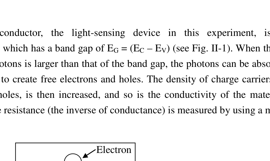
Fig. II-1. Schematic diagram of an electron-hole pair generated by a single photon in a semiconductor. ($E_V$ = Valence Band Edge; $E_G$ = Energy Gap; $E_C$ = Conduction Band Edge.)

In the semiconductor laser, the light emitting device in this experiment, as the external source injects electrons and holes into the device, they can combine to emit photons as shown schematically in the Fig. II-2. Ideally, the combination of one pair of electron and hole can generate one photon. Realistically, there are also nonradiative processes through which an electron-hole pair recombines without generating a photon. Thus the number of photons generated is not equal to the number of electron-hole pairs recombined. The average fractional number of photons generated by an electron-hole pair is called the quantum efficiency.

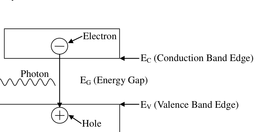
Fig. II-2. Schematic diagram of a single photon generated by an electron-hole pair combined in a semiconductor. ($E_C$ = Conduction Band Edge; $E_V$ = Valence Band Edge; $E_G$ = Energy Gap.)

The semiconductor laser can emit a monochromatic, partially polarized and coherent light beam. The partially polarized light is composed of two parts – linearly polarized and unpolarized. The light intensity due to the former is denoted by $J_p$ and the other by $J_u$. When the partially polarized light is incident upon a polarizer, the transmittance of the linearly polarized part depends on the angle between its polarized direction and the direction of the polarizer. But for the unpolarized part, a constant portion is allowed to pass through the polarizer and is independent of the angle.

Experiments and Procedures

Exp. II-A. Light Response of the Photoconductor

The light source used in this part should be the collimated laser diode (CLD). Use the circuit diagram shown in Fig. IIA-1 to provide current for the CLD. The symbols used in Fig. IIA-1 are listed in Table IIA-1.

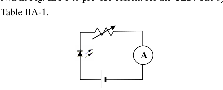
Fig. IIA-1. Circuit diagram used for the CLD.

Table IIA-1. Symbols used in Fig. IIA-1

Devices	Collimated Laser Diode	5V dc-power	Variable Resistors	Ammeter (Multimeter)
Label	C-C-#	C-D-#	C-E-#	II-X, II-Y

Operate the CLD with the maximum current. The laser intensity is detected by a photoconductor (PC). When you shine light on a PC, the conductance increases with the light intensity. You should minimize the ambient light effect. In this experiment, we actually measure the resistance, which is the inverse of conductance. The intensity of the laser light reaching the PC may be varied by using the supplied polarizers or filters. The symbols of other optical components are given in the Table IIA-2. The partial polarization of the laser light may be observed by using the experimental setup in the Fig. IIA-2.

Table IIA-2. Symbols of optical components.

Devices	Collimated Laser Diode	Polarizers	Photoconductor	Light filter
Symbol label	L	P1, P2	PC	F (Optional)
Label	C-C-#	II-P-#, II-Q-#	II-W-#	II-U

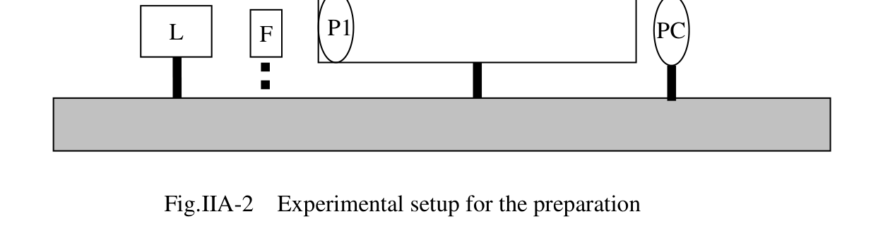
Fig. IIA-2. Experimental setup for the preparation.

Rotating P1, one should observe that the PC resistance varies. Adjust P1 so that the PC resistance reaches a minimum. If the observed minimum resistance happens in a range, say $10^{\circ }$ or larger of the rotation angle of P1, then the PC is saturated. In this case light filter(s) should be used to avoid PC saturation near the maximum light intensity.

Fix the P1 position according to the description in previous paragraph. Characterize the conductance of the PC versus the relative light intensity following the experimental setup shown in the Fig. IIA-3.

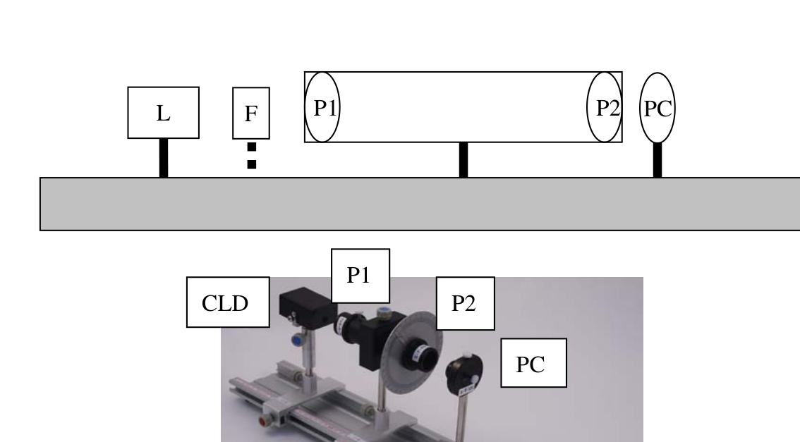
Fig. IIA-3. Experimental setup for the PC characterization.

(1) Define ${\theta }_P$ to be the relative angle between polarization axes of P1 and P2. By varying the angle ${\theta }_P$ from $0^{\circ }$ to $180^{\circ }$ in step of $5^{\circ }$. Record the measured PC resistance and ${\theta }_P$ in the data table. Transform the measured PC resistance values into conductance values and record them in the data table. No error analysis is required. (1.2 points)

(2) Plot the PC conductance values as a function of ${\theta }_P$ on a graph paper. No error analysis is required. (1.2 points)

Exp. II-B. The Fraction of Linearly Polarized Laser Light

The light source used in this part should be the collimated laser diode (CLD) with a 15 mA current from the dc power supply. The task in this part is to determine the fraction $\beta$ of the laser light that is linearly polarized by using the setup in Fig. IIA-2, which is the same as the previous section. No error analysis is required in this part.

$\beta =\frac{J(\text{Linearly Polarized})}{J(\text{Unpolarized})+J(\text{Linearly Polarized})}=\frac{J_{max}-J_{min}}{J_{max}+J_{min}}$

$J_{max}$ and $J_{min}$ are the maximum and minimum light intensity detected by PC while rotating P1.

Fig. IIA-2. Experimental setup for the preparation.

(1) Find the maximum and minimum values of PC resistance ($R_{max}$ and $R_{min}$) by rotating P1 $360^{\circ }$. Transform $R_{max}$ and $R_{min}$ into the minimum and maximum values of PC conductance $C_{min}$ and $C_{max}$. Record the data in the data table. (0.8 points)

(2) Utilizing the conductance versus ${\theta }_P$ graph in Exp. II-A-(2) to determine the relative intensities $J_{max}$ and $J_{min}$ corresponding to $C_{max}$ and $C_{min}$. Write down the result on the answer sheet. (1.6 points)

(3) Calculate $\beta$ and write down the result on the answer sheet. (0.2 points)

Exp. II-C. The Differential Quantum Efficiency of the Collimated Laser Diode

The task of this part is to characterize the relative light intensity versus the current through the collimated laser diode (CLD) and determine the Differential Quantum Efficiency $\eta$, which will be defined below. Control the current of CLD in the range between 5 mA and 20 mA. Make sure that the PC is not saturated when the current is close to 20 mA. Filters or polarizers can be used to avoid saturation.

(1) Control the CLD current and measure the corresponding PC resistance values. Record the data in the data table. Transform your data and plot the PC conductance versus CLD current on a graph paper. No error analysis is required. (1.3 points)

(2) Based on the graph of step (1), choose a region ($\Delta I\sim 3$ mA) centered around the maximum slope. By using the conductance versus ${\theta }_P$ graph in Part II-A-(2), transform and record the data of this region in the table of step (1) into the relative light intensity ($J$). Plot the relative light intensity ($J$) versus CLD current ($I$) on a graph paper. No error analysis is required. (0.8 points)

(3) The maximum radiating power of the CLD is assumed to be exactly $P_{max}=3.0$ mW. Extract the maximum slope from the graph in step (2) and transfer it to the value of $G\equiv \frac{\Delta P_{max}}{\Delta I}$, which is the maximum ratio of the increased amount of radiating power and the increase amount of input current. Write down your analysis and the calculated value $G$ on the answer sheet. Estimate the error of $G$. Do not include the error of the $P_{max}$. Write down your analysis and the calculated value $\Delta G$ on the answer sheet. (2.0 points)

(4) The Quantum Efficiency equals the probability of one photon being generated per electron injected. From a particular bias current of the laser, a small increment of electrons injected would cause a corresponding increment of photons. The Differential Quantum Efficiency $\eta$ is defined as the ratio of the increased number of photons and the increased number of injected electrons. Determine $\eta$ of your CLD by using the value of $G$ obtained in step (3). Write down your analysis and the calculated value $\eta$ on the answer sheet. Estimate the error of $\eta$. Write down your analysis and the calculated value $\Delta \eta$ on the answer sheet. (Laser wavelength = 650 nm. Planck’s constant = $6.63\times 10^{-34}\text{J}\cdot \text{s}$. Light speed = $3.0\times 10^8\text{m/s}$.) (0.9 points)

Fonte: Testo (PDF) — p.1 Topic: Modern-Quantum Physics, Wave Optics Metodi: Experimental Data Analysis, Photon Energy Relation, Graph Linearization, Error Propagation Competenze: Experimental Data Analysis, Measurement & Instrumentation, Curve Fitting, Error Propagation Objects: Photon, Electron

Esperimento II. Comprendere i laser semiconduttori

Lo scopo di questo esperimento è quello di esplorare le caratteristiche di base dei laser semiconduttori. Misureremo e calcoleremo la frazione della polarizzazione lineare del raggio laser collimato utilizzando un paio di polarizzatori e un fotoconduttore. Infine, determineremo il valore massimo dell’aumento di potenza per incremento corrente del laser collimato.

Attenzione: non guardare direttamente il raggio laser, che può danneggiare gli occhi!!

Descrizione di sfondo

Il fotoconduttore, il dispositivo di rilevamento della luce di questo esperimento, è costituito da semiconduttore, che ha un intervallo di banda di $E_G=(E_C-E_V)$ (vedi figura 1. II-1). Quando l’energia dei fotoni incidenti è maggiore di quella del gap di banda, i fotoni possono essere assorbiti dal semiconduttore per creare elettroni e fori liberi. La densità dei vettori di carica, compresi elettroni e fori, aumenta quindi, così come la conducibilità del materiale. In questo esperimento, la resistenza (l’inverso della conduttività) viene misurata utilizzando un multimetro.

• Non è vero. II-1. Diagramma schematico di una coppia di fori elettronici generata da un singolo fotone in un semiconduttore.](../_attaccamenti/APhO_2010_exp/APhO_2010_exp_Q2_p1_f1.png)

Fig. - Cosa? II-1. Diagramma schematico di una coppia di fori elettronici generata da un singolo fotone in un semiconduttore. ($E_V$ = Valence Band Edge; $E_G$ = Gap di energia; $E_C$ = Edge di banda di condotta.)

Nel laser semiconduttore, il dispositivo emettente luce in questo esperimento, come la fonte esterna inietta elettroni e fori nel dispositivo, possono combinarsi per emettere fotoni come mostrato schematicamente nella figura. II-2. Idealmente, la combinazione di un paio di elettroni e di buchi può generare un fotone. Realmente, ci sono anche processi non irradiativi attraverso i quali una coppia di buchi elettronici ricombina senza generare un fotone. Quindi il numero di fotoni generati non è uguale al numero di coppie di fori elettronici ricombinati. Il numero frazionario medio di fotoni generati da una coppia di fori elettronici è chiamato efficienza quantistica.

• Non è vero. II-2. Schematico di un singolo fotone generato da una coppia di fori elettronici combinata in un semiconduttore.](../_attaccamenti/APhO_2010_exp/APhO_2010_exp_Q2_p2_f1.png)

Fig. - Cosa? II-2. Diagramma schematico di un singolo fotone generato da una coppia di fori elettronici combinata in un semiconduttore. ($E_C$ = bordo della banda di condotta; $E_V$ = bordo della banda di valenza; $E_G$ = distanza energetica.)

Il laser semiconduttore può emettere un raggio di luce monocromatico, parzialmente polarizzato e coerente. La luce parzialmente polarizzata è composta da due parti linearmente polarizzata e non polarizzata. L’intensità luminosa dovuta alla prima è indicata da $J_p$ e all’altra da $J_u$. Quando la luce parzialmente polarizzata incide su un polarizzatore, la trasmissione della parte polarizzata lineare dipende dall’angolo tra la sua direzione polarizzata e la direzione del polarizzatore. Ma per la parte non polarizzata, una porzione costante è consentita di passare attraverso il polarizzatore ed è indipendente dall’angolo.

Esperimenti e procedure

• Esplosione. II-A. Risposta alla luce del fotoconduttore

La fonte luminosa utilizzata in questa parte dovrebbe essere la dioda laser collimata (CLD). Utilizzare il diagramma di circuito mostrato nella figura. IIA-1 per fornire corrente per il CLD. I simboli utilizzati in Figura. IIA-1 sono elencati nella tabella IIA-1.

• Non è vero. IIA-1. Diagramma di circuito utilizzato per il CLD.](../_attaccamenti/APhO_2010_exp/APhO_2010_exp_Q2_p3_f1.png)

Fig. - Cosa? IIA-1. Diagramma di circuito utilizzato per il CLD.

Tabella IIA-1. I simboli utilizzati in Fig. IIA-1

♬ Dispositivi ♬ Diodo laser collimato ♬ Potenza di 5V DC ♬ Resistori variabili ♬ Ammetro (Multimetro) ♬ |---|---|---|---|---|

# Taglio C-C-# # C-D-# # C-E-# # II-X, II-Y

Operare il CLD con la corrente massima. L’intensità laser è rilevata da un fotoconduttore (PC). Quando si illumina un PC, la conduttività aumenta con l’intensità della luce. Dovresti ridurre al minimo l’effetto di luce ambientale. In questo esperimento, misuriamo la resistenza, che è l’inverso della conduttività. L’intensità della luce laser che raggiunge il PC può essere variata utilizzando i polarizzatori o i filtri forniti. I simboli di altri componenti ottici sono riportati nella tabella IIA-2. La polarizzazione parziale della luce laser può essere osservata utilizzando l’impostazione sperimentale riportata nella figura. IIA-2.

Tabella IIA-2. I simboli dei componenti ottici.

Dispositivi Diodo Laser Collimato Polarizzatori Fotoconduttore Filtro luce |---|---|---|---|---| Simbolo etichetta L P1, P2 PC F (Optional)

Il taglio C-C-# # II-P-#, II-Q-# # II-W-#

• Non è vero. IIA-2. L’impiego di un’unità di controllo di controllo è stato effettuato in base al metodo di controllo.

Fig. - Cosa? IIA-2. La preparazione è stata organizzata in modo sperimentale.

Per la rotazione P1, si deve osservare che la resistenza PC varia. Aggiusta P1 in modo che la resistenza del PC raggiunga il minimo. Se la resistenza minima osservata si verifica in un intervallo, ad esempio $10^{\circ }$ o superiore all’angolo di rotazione di P1, allora il PC è saturo. In questo caso, è necessario utilizzare un filtro luminoso (s) per evitare la saturazione del PC vicino all’intensità massima della luce.

Rettifica la posizione P1 secondo la descrizione del paragrafo precedente. Caratterizzare la conduttività del PC rispetto all’intensità relativa della luce dopo l’impostazione sperimentale mostrata nella figura. IIA-3.

• Non è vero. IIA-3. Configurazione sperimentale per la caratterizzazione del PC.](../_attaccamenti/APhO_2010_exp/APhO_2010_exp_Q2_p5_f1.png)

Fig. - Cosa? IIA-3. Configurazione sperimentale per la caratterizzazione del PC.

**(1) ** Definire ${\theta }_P$ come angolo relativo tra gli assi di polarizzazione di P1 e P2. Variando l’angolo ${\theta }_P$ da $0^{\circ }$ a $180^{\circ }$ in passo $5^{\circ }$. Registrare la resistenza misurata del PC e ${\theta }_P$ nella tabella dei dati. Trasformare i valori di resistenza del PC misurati in valori di conduttività e registrarli nella tabella dati. Non è necessaria alcuna analisi degli errori. *(1,2 punti) *

**(2) ** Tracciare i valori di conduttività del PC come funzione di ${\theta }_P$ su una carta grafica. Non è necessaria alcuna analisi degli errori. *(1,2 punti) *

• Esplosione. II-B. La frazione della luce laser polarizzata lineare

La fonte luminosa utilizzata in questa parte deve essere la dioda laser collimata (CLD) con una corrente di 15 mA proveniente dalla alimentazione di corrente continua. Il compito di questa parte è determinare la frazione $\beta$ della luce laser polarizzata linearmente utilizzando l’impostazione di cui alla figura. IIA-2, che è la stessa sezione precedente. Non è richiesta alcuna analisi degli errori in questa parte.

$\beta =\frac{J(\text{Linearly Polarized})}{J(\text{Unpolarized})+J(\text{Linearly Polarized})}=\frac{J_{max}-J_{min}}{J_{max}+J_{min}}$

$J_{max}$ e $J_{min}$ sono l’intensità massima e minima di luce rilevata dal PC durante la rotazione di P1.

• Non è vero. IIA-2. L’impiego di un’unità di controllo di controllo è stato effettuato in base al metodo di controllo.

Fig. - Cosa? IIA-2. La preparazione è stata organizzata in modo sperimentale.

**(1) ** Trovare i valori massimi e minimi della resistenza PC ($R_{max}$ e $R_{min}$) rotando P1 $360^{\circ }$. Trasformare $R_{max}$ e $R_{min}$ in valori minimi e massimi di conduttività del PC $C_{min}$ e $C_{max}$. Registrare i dati nella tabella dati. *(0,8 punti) *

**(2) ** Utilizzando la conduttività contro ${\theta }_P$ grafico in Exp. II-A-(2) per determinare le intensità relative $J_{max}$ e $J_{min}$ corrispondenti a $C_{max}$ e $C_{min}$. Scrivi il risultato sulla scheda delle risposte. *(1,6 punti) *

**(3) ** Calcolare $\beta$ e scrivere il risultato sulla scheda delle risposte. *(0,2 punti) *

• Esplosione. II-C. L’efficienza quantistica differenziale della dioda laser collimata

Il compito di questa parte è quello di caratterizzare l’intensità relativa della luce rispetto alla corrente attraverso il diodo laser collimato (CLD) e determinare l’efficienza quantistica differenziale $\eta$, che sarà definita di seguito. Controllare la corrente di CLD nell’intervallo tra 5 mA e 20 mA. Assicurarsi che il PC non sia saturo quando la corrente è vicina a 20 mA. Per evitare la saturazione possono essere utilizzati filtri o polarizzatori.

**(1) ** Controlla la corrente CLD e misura i valori di resistenza PC corrispondenti. Registrare i dati nella tabella dati. Trasforma i dati e disegna la conduttività del PC contro la corrente CLD su una carta grafica. Non è necessaria alcuna analisi degli errori. *(1,3 punti) *

**(2) ** Sulla base del grafico di passo (1), scegliere una regione ($\Delta I\sim 3$ mA) incentrata intorno alla pendice massima. Utilizzando il grafico di conduttività contro ${\theta }_P$ nella parte II-A-(2), trasforma e registra i dati di questa regione nella tabella del passo (1) in intensità relativa della luce ($J$). Tracciare l’intensità relativa della luce ($J$) rispetto alla corrente CLD ($I$) su una carta grafica. Non è necessaria alcuna analisi degli errori. *(0,8 punti) *

**(3) ** Si presume che la potenza radiante massima del CLD sia esattamente $P_{max}=3.0$ mW. Estrazione della pendenza massima dal grafico in fase (2) e trasferimento al valore di $G\equiv \frac{\Delta P_{max}}{\Delta I}$, che è il rapporto massimo tra l’aumento della potenza radiante e l’aumento della corrente di ingresso. Scrivi la tua analisi e il valore calcolato $G$ sulla scheda delle risposte. Calcolare l’errore di $G$. Non include l’errore di $P_{max}$. Scrivi la tua analisi e il valore calcolato $\Delta G$ sulla scheda delle risposte. *(2,0 punti) *

**(4) ** L’efficienza quantistica è uguale alla probabilità che un fotone venga generato per ogni elettrone iniettato. Da una particolare corrente di bias del laser, un piccolo incremento di elettroni iniettati causerebbe un corrispondente incremento di fotoni. L’efficienza quantistica differenziale $\eta$ è definita come il rapporto tra l’aumento del numero di fotoni e l’aumento del numero di elettroni iniettati. Determina il $\eta$ della tua DCC utilizzando il valore di $G$ ottenuto nella fase (3). Scrivi la tua analisi e il valore calcolato $\eta$ sulla scheda delle risposte. Calcolare l’errore di $\eta$. Scrivi la tua analisi e il valore calcolato $\Delta \eta$ sulla scheda delle risposte. (Lenghe d’onda laser = 650 nm. Costante di Planck = $6.63\times 10^{-34}\text{J}\cdot \text{s}$. Velocità della luce = $3.0\times 10^8\text{m/s}$.) *(0,9 punti) *

Fonte: Testo (PDF) — p.1 Topic: Modern-Quantum Physics, Wave Optics Metodi: Experimental Data Analysis, Photon Energy Relation, Graph Linearization, Error Propagation Competenze: Experimental Data Analysis, Measurement & Instrumentation, Curve Fitting, Error Propagation Objects: Photon, Electron