APhO 2010 — Teorica

Theoretical Question 1 — Particles and Waves

This question includes the following three parts dealing with motions of particles and waves:

• Part A. Inelastic scattering of particles
• Part B. Waves on a string
• Part C. Waves in an expanding universe

Part A. Inelastic Scattering and Compositeness of Particles

A particle is considered elementary if it has no excitable internal degrees of freedom such as, for example, rotations and vibrations about its center of mass. Otherwise, it is composite.

To determine if a particle is composite, one may set up a scattering experiment with the particle being the target and allow an elementary particle to scatter off it. In case that the target particle is composite, the scattering experiment may reveal important features such as scaling, i.e. as the forward momentum of the scattered particle increases, the scattering cross section becomes independent of the momentum.

For a scattering system consisting of an elementary particle incident on a target particle, we shall denote by $Q$ the total translational kinetic energy loss of the system. Here the translational kinetic energy of a particle, whether elementary or composite, is defined as the kinetic energy associated with the translational motion of its center of mass. Thus we may write

$Q=K_i-K_f,$

where $K_i$ and $K_f$ are the total translational kinetic energies of the scattering pair before and after scattering, respectively.

In Part A, use non-relativistic classical mechanics to solve all problems. All effects due to gravity are to be neglected.

(a) As shown in Fig. 1, an elementary particle of mass $m$ moves along the $x$ axis with $x$-component of momentum $p_1>0$. After being scattered by a stationary target of mass $M$, its momentum becomes ${\vec{p}}_2$.

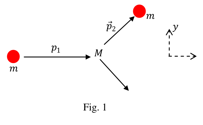
Fig. 1

From data on ${\vec{p}}_2$, one can determine if the target particle is elementary or composite. We shall assume that ${\vec{p}}_2$ lies in the $x$-$y$ plane and that the $x$- and $y$-components of ${\vec{p}}_2$ are given, respectively, by $p_{2x}$ and $p_{2y}$.

(i) Find an expression for $Q$ in terms of $m$, $M$, $p_1$, $p_{2x}$, and $p_{2y}$. [0.2 point]

(ii) If the target particle is elementary, the momenta $p_1$, $p_{2x}$, and $p_{2y}$ are related in a particular way by a condition.

For given $p_1$, plot the condition as a curve in the $p_{2x}$-$p_{2y}$ plane. Specify the value of $p_{2x}$ for each intercept of the curve with the $p_{2x}$-axis. In the same plot, locate regions of points of ${\vec{p}}_2$ corresponding to $Q<0$, $Q=0$, $Q>0$, and label each of them as such. [0.7 point]

For a stationary composite target in its ground state before scattering, which region(s) of $Q$ contains those points of ${\vec{p}}_2$ allowed? [0.2 point]

(b) Now, consider a composite target consisting of two elementary particles each with mass $\frac{1}{2}M$. They are connected by a spring of negligible mass. See Fig. 2. The spring has a force constant $k$ and does not bend sideways. Initially, the target is stationary with its center of mass at the origin $O$, and the spring, inclined at an angle $\theta$ to the $x$-axis, is at its natural length $d_0$. For simplicity, we assume that only vibrational and rotational motions can be excited in the target as a result of scattering.

The incident elementary particle of mass $m$ moves in the $x$-direction both before and after scattering with its momenta given, respectively, by $p_1$ and $p_2$. Note that $p_2$ is negative if the particle recoils and moves backward. A scattering occurs only if the incident particle hits one of the target particles and $p_2\ne p_1$. We assume all three particles move in the same plane before and after scattering.

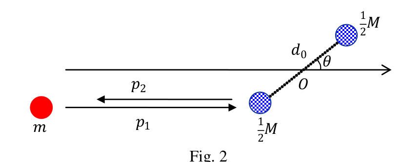
Fig. 2

(i) If the maximum length of the spring after scattering is $d_m$, find an equation which relates the ratio $x=(d_m-d_0)/d_0$ to the quantities $Q$, $\theta$, $d_0$, $m$, $k$, $M$, $p_1$ and $p_2$. [0.7 point]

(ii) Let $\alpha \equiv {\sin }^2\theta$. When the angle of orientation $\theta$ of the target is allowed to vary, the scattering cross section $\sigma$ gives the effective target area, in a plane normal to the direction of incidence, which allows certain outcomes to occur as a result of scattering. It is known that for all outcomes which lead to the same value of $p_2$, the value of $\alpha$ must span an interval $({\alpha }_{\min },{\alpha }_{\max })$ and we may choose the unit of cross section so that $\sigma$ is simply given by the numerical range $({\alpha }_{\max }-{\alpha }_{\min })$ of the interval. Note that ${\alpha }_{\min }$, ${\alpha }_{\max }$, and, consequently, $\sigma$ are dependent on $p_2$. Let $p_c$ be the threshold value of $p_2$ at which $\sigma$ starts to become independent of $p_2$.

In the limit of large $k$, give an estimate of $p_c$. Express your answer in terms of $m$, $M$, and $p_1$. [1.1 points]

Assume $M=3m$ and in the limit of large $k$, plot $\sigma$ as a function of $p_2$ for a given $p_1$. In the plot, specify the range of $\sigma$ and $p_2$. [1.1 points]

Part B. Waves on a String

Consider an elastic string stretched between two fixed ends A and B, as shown in Fig. 3. The linear mass density of the string is $\mu$. The speed of propagation for transverse waves in the string is $c$. Let the length $\overline{AB}$ be $L$. The string is plucked sideways and held in a triangular form with a maximum height $h\ll L$ at its middle point. At time $t=0$, the plucked string is released from rest. All effects due to gravity may be neglected.

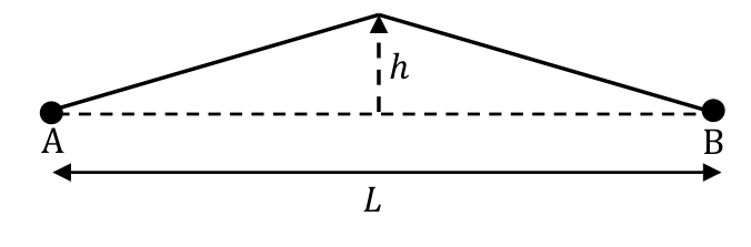
Fig. 3

(c) Find the period of vibration $T$ for the string. [0.5 point]

Plot the shape of the string at $t=T/8$. In the plot, specify lengths and angles which serve to define the shape of the string. [1.7 points]

(d) Find the total mechanical energy of the vibrating string in terms of $\mu$, $c$, $h$, and $L$. [0.8 point]

Part C. An Expanding Universe

Photons in the universe play an important role in delivering information across the cosmos. However, the fact that the universe is expanding must be taken into account when one tries to extract information from these photons. To this end, we normally express length and distance using a universal scale factor $a(t)$ which depends on time $t$. Thus the distance $L(t)$ between two stars stationary in their respective local frames is proportional to $a(t)$:

L(t) = ka(t), \tag{1}

where $k$ is a constant and $a(t)$ accounts for the expansion of the universe. We use a dot above a symbol of a variable to denote its time derivative, i.e. $\dot{a}(t)=da(t)/dt$, and let $v(t)\equiv \dot{L}(t)$. Taking time derivatives of both sides of Eq. (1), one obtains the Hubble law:

v(t) = H(t)L(t), \tag{2}

where $H(t)=\dot{a}(t)/a(t)$ is the Hubble parameter at time $t$. At the current time $t_0$, we have

$H(t_0)=72\mathrm{km}{\mathrm{s}}^{-1}\mathrm{Mp}{\mathrm{c}}^{-1},$

where $1\mathrm{Mpc}=3.0857\times 10^{19}\mathrm{km}=3.2616\times 10^6$ light-year.

Assume the universe to be infinitely large and expanding in such a way that

$a(t)\propto \exp (bt),$

where $b$ is a constant. In such a universe, the Hubble parameter is a constant equal to $H(t_0)$. Moreover, it can be shown that the wavelength $\lambda$ of photons travelling in the universe will be stretched in proportion to the expansion of the universe, i.e.

$\lambda (t)\propto a(t).$

Now suppose that photons making up a Lyman-alpha emission line were emitted at $t_e$ by a star that was stationary in its local frame and that we as observers are stationary in our local frame. When these photons were emitted, their wavelength was $\lambda (t_e)=121.5\mathrm{nm}$. But when they reach us now at $t_0$, their wavelength is red-shifted to $145.8\mathrm{nm}$.

(e) As these photons traveled, the universe kept expanding so that the star kept receding from us. Given that the speed of light in vacuum $c$ has never changed, what was the distance $L(t_e)$ of the star from us when these photons were emitted at $t_e$? Express the answer in units of Mpc. [2.2 points]

(f) What is the receding velocity $v(t_0)$ of the star with respect to us now at $t_0$? Express the answer in units of the speed of light in vacuum $c$. [0.8 point]

Appendix

The following formula may be used when needed:

${\int }_a^b{e}^{\beta x}dx=\frac{1}{\beta }\left(e^{\beta b}-e^{\beta a}\right).$

Fonte: Testo (PDF) — p.1

Topic: Conservation of Momentum, Oscillations & Waves, Astrophysics Metodi: Conservation of Momentum, Conservation of Energy, Wave Equation, Calculus-Integration Competenze: Physical Reasoning, Mathematical Modeling, Diagrammatic Reasoning Objects: Spring, String, Photon

Domanda teorica 1 Particelle e onde

Questa domanda comprende le seguenti tre parti che riguardano i movimenti delle particelle e delle onde:

• Parte A. Distraggio inelastico delle particelle
• Parte B. onde su una corda
• Parte C. Le onde in un universo in espansione

Parte A. Distribuzione e composizione delle particelle inelastica

Una particella è considerata elementare se non ha gradi interni eccitabili di libertà come, ad esempio, rotazioni e vibrazioni intorno al suo centro di massa. In caso contrario, è composto.

Per determinare se una particella è composta, si può impostare un esperimento di dispersione con la particella come obiettivo e permettere a una particella elementare di disperdersi da essa. Nel caso in cui la particella di destinazione sia composta, l’esperimento di dispersione può rivelare caratteristiche importanti come scaling, cioè a misura che la velocità di avanzamento della particella dispersa aumenta, la sezione trasversale di dispersione diventa indipendente dalla velocità.

Per un sistema di dispersione costituito da un incidente di particelle elementari su una particella di destinazione, si indica con $Q$ la perdita totale di energia cinetica traslazionale del sistema. Qui l’energia cinetica traslazionale di una particella, elementare o composta, è definita come l’energia cinetica associata al movimento traslazionale del suo centro di massa. Così possiamo scrivere

$Q=K_i-K_f,$

dove $K_i$ e $K_f$ sono rispettivamente le energie cinetiche traslazionali totali della coppia di dispersione prima e dopo la dispersione.

Nella parte A, utilizzare la meccanica classica non relativistica per risolvere tutti i problemi. Tutti gli effetti dovuti alla gravità devono essere trascurati.

**(a) ** Come mostrato alla figura. 1, una particella elementare di massa $m$ si muove lungo l’asse $x$ con $x$-componente di impulso $p_1>0$. Dopo essere stato disperso da un obiettivo stazionario di massa $M$, il suo impulso diventa ${\vec{p}}_2$.

Fig. 1

Dalle informazioni su ${\vec{p}}_2$ si può determinare se la particella di destinazione è elementare o composta. Presumere che ${\vec{p}}_2$ si trovi nel piano $x$-$y$ e che i componenti $x$- e $y$ di ${\vec{p}}_2$ siano dati rispettivamente da $p_{2x}$ e $p_{2y}$.

**(i) ** Trova un’espressione per $Q$ in termini di $m$, $M$, $p_1$, $p_{2x}$ e $p_{2y}$. [0,2 punto]

(ii) If the target particle is elementary, the momenta $p_1$, $p_{2x}$, and $p_{2y}$ are related in a particular way by a condition.

Per un dato $p_1$, tracciare la condizione come curva nel piano $p_{2x}$-$p_{2y}$. Indicare il valore di $p_{2x}$ per ogni intersezione della curva con l’asse $p_{2x}$. Nella stessa superficie, individuare le regioni di punti ${\vec{p}}_2$ corrispondenti a $Q<0$, $Q=0$, $Q>0$ e etichettarne ciascuno come tale. [0,7 punto]

Per un bersaglio composto stazionario nel suo stato di base prima della dispersione, quale regione di $Q$ contiene i punti di ${\vec{p}}_2$ consentiti? [0,2 punto]

**(b) ** Ora, consideriamo un obiettivo composto costituito da due particelle elementari ognuna con massa $\frac{1}{2}M$. Sono collegate da una sorgente di massa trascurabile. Vedi Fig. 2. La molla ha una costante di forza $k$ e non si piega lateralmente. Inizialmente, l’obiettivo è stazionario con il suo centro di massa all’origine $O$, e la molla, inclinata ad un angolo $\theta$ all’asse $x$, è alla sua lunghezza naturale $d_0$. Per semplicità, supponiamo che solo i movimenti vibrazionali e di rotazione possano essere eccitati nell’obiettivo a seguito della dispersione.

La particella elementare incidente di massa $m$ si muove nella direzione $x$ sia prima che dopo la dispersione con il suo momento dato rispettivamente da $p_1$ e $p_2$. Nota che $p_2$ è negativo se la particella si ritira e si muove indietro. Una dispersione si verifica solo se la particella incidentale colpisce una delle particelle bersaglio e $p_2\ne p_1$. Supponiamo che tutte e tre le particelle si muovano nello stesso piano prima e dopo la dispersione.

Fig. 2

(i) If the maximum length of the spring after scattering is $d_m$, find an equation which relates the ratio $x=(d_m-d_0)/d_0$ to the quantities $Q$, $\theta$, $d_0$, $m$, $k$, $M$, $p_1$ and $p_2$. [0,7 punto]

**(ii) ** Lasciate $\alpha \equiv {\sin }^2\theta$. Quando l’angolo di orientamento $\theta$ dell’obiettivo è consentito di variare, la sezione trasversale di dispersione $\sigma$ dà l’area di destinazione effettiva, in un piano normale alla direzione di incidenza, che consente di ottenere determinati risultati a seguito della dispersione. È noto che per tutti i risultati che portano allo stesso valore di $p_2$, il valore di $\alpha$ deve coprire un intervallo $({\alpha }_{\min },{\alpha }_{\max })$ e possiamo scegliere l’unità di sezione incrociata in modo che $\sigma$ sia semplicemente data dall’intervallo numerico $({\alpha }_{\max }-{\alpha }_{\min })$ dell’intervallo. Si noti che ${\alpha }_{\min }$, ${\alpha }_{\max }$ e, di conseguenza, $\sigma$ dipendono da $p_2$. Il valore $p_c$ deve essere il valore soglia di $p_2$ al quale $\sigma$ inizia a diventare indipendente da $p_2$.

Nel limite di grande $k$, indicare una stima di $p_c$. Esprimere la risposta in termini di $m$, $M$ e $p_1$. [1.1 punti]

Supponiamo $M=3m$ e nel limite di grande $k$, il plot $\sigma$ come funzione di $p_2$ per un dato $p_1$. Nella figura, specificare l’intervallo di $\sigma$ e $p_2$. [1.1 punti]

Parte B. Le onde su una corda

Considerate una corda elastica estesa tra due estremità fisse A e B, come mostrato nella figura. 3. La densità di massa lineare della stringa è $\mu$. La velocità di propagazione per le onde trasversali nella corda è $c$. La lunghezza $\overline{AB}$ deve essere $L$. La corda è strappata lateralmente e tenuta in forma triangolare con un’altezza massima $h\ll L$ al suo punto medio. Al tempo $t=0$, la corda strappata viene rilasciata dal riposo. Tutti gli effetti dovuti alla gravità possono essere trascurati.

Fig. 3

**(c) ** Trova il periodo di vibrazione $T$ per la corda. [0,5 punto]

Tracciare la forma della stringa a $t=T/8$. Nella trama, specificare lunghezze e angoli che servono a definire la forma della corda. [1,7 punti]

**(d) ** Trova l’energia meccanica totale della corda vibrante in termini di $\mu$, $c$, $h$ e $L$. [0,8 punto]

Parte C. Un universo in espansione

I fotoni nell’universo svolgono un ruolo importante nel trasmettere informazioni attraverso il cosmo. Tuttavia, il fatto che l’universo si stia espandendo deve essere preso in considerazione quando si tenta di estrarre informazioni da questi fotoni. A tal fine, normalmente si esprimono lunghezza e distanza utilizzando un fattore di scala universale $a(t)$ che dipende dal tempo $t$. La distanza $L(t)$ tra due stelle stazionarie nei rispettivi quadri locali è quindi proporzionale a $a(t)$:

L(t) = ka(t), \tag{1}

dove $k$ è una costante e $a(t)$ rappresenta l’espansione dell’universo. Usiamo un punto sopra un simbolo di una variabile per indicare la sua derivata temporale, cioè $\dot{a}(t)=da(t)/dt$, e lasciate $v(t)\equiv \dot{L}(t)$. Prendendo derivati temporali di entrambe le parti di Eq. (1), si ottiene la legge di Hubble:

v(t) = H(t)L(t), \tag{2}

dove $H(t)=\dot{a}(t)/a(t)$ è il parametro Hubble al tempo $t$. Al momento attuale $t_0$, abbiamo

$H(t_0)=72\mathrm{km}{\mathrm{s}}^{-1}\mathrm{Mp}{\mathrm{c}}^{-1},$

dove $1\mathrm{Mpc}=3.0857\times 10^{19}\mathrm{km}=3.2616\times 10^6$ anno luce.

Supponiamo che l’universo sia infinitamente grande ed espande in modo tale che

$a(t)\propto \exp (bt),$

in cui $b$ è una costante. In un tale universo, il parametro di Hubble è una costante uguale a $H(t_0)$. Inoltre, si può dimostrare che la lunghezza d’onda $\lambda$ dei fotoni che viaggiano nell’universo sarà estesa in proporzione all’espansione dell’universo, cioè

$\lambda (t)\propto a(t).$

Supponiamo che i fotoni che compongono una linea di emissioni Lyman-alpha siano stati emessi a $t_e$ da una stella che era stazionaria nel suo quadro locale e che noi come osservatori siamo stazionari nel nostro quadro locale. Quando questi fotoni sono stati emessi, la loro lunghezza d’onda è stata $\lambda (t_e)=121.5\mathrm{nm}$. Ma quando ci raggiungono ora a $t_0$, la loro lunghezza d’onda è spostata in rosso a $145.8\mathrm{nm}$.

(e) As these photons traveled, the universe kept expanding so that the star kept receding from us. Given that the speed of light in vacuum $c$ has never changed, what was the distance $L(t_e)$ of the star from us when these photons were emitted at $t_e$? Esprimere la risposta in unità di Mpc. [2,2 punti]

(f) What is the receding velocity $v(t_0)$ of the star with respect to us now at $t_0$? Esprimere la risposta in unità della velocità della luce nel vuoto $c$. [0,8 punto]

Appendice

Se necessario, può essere utilizzata la seguente formula:

${\int }_a^b{e}^{\beta x}dx=\frac{1}{\beta }\left(e^{\beta b}-e^{\beta a}\right).$

Fonte: Testo (PDF) — p.1

Topic: Conservation of Momentum, Oscillations & Waves, Astrophysics Metodi: Conservation of Momentum, Conservation of Energy, Wave Equation, Calculus-Integration Competenze: Physical Reasoning, Mathematical Modeling, Diagrammatic Reasoning Objects: Spring, String, Photon

Theoretical Question 2 — Strong Resistive Electromagnets

Resistive electromagnets are magnets with coils made of a normal metal such as copper or aluminum. Modern strong resistive electromagnets can provide steady magnetic fields higher than 30 tesla. Their coils are typically built by stacking hundreds of thin circular plates made of copper sheet metal with lots of cooling holes stamped in them; there are also insulators with the same pattern. When voltage is applied across the coil, current flows through the plates along a helical path to generate high magnetic fields in the center of the magnet.

In this question we aim to assess if a cylindrical coil (or solenoid) of many turns can serve as a magnet for generating high magnetic fields. As shown in Fig. 1, the center of the magnet is at $O$. Its cylindrical coil consists of $N$ turns of copper wire carrying a current $I$ uniformly distributed over the cross section of the wire. The coil’s mean diameter is $D$ and its length along the axial direction $x$ is $\ell$. The wire’s cross section is rectangular with width $a$ and height $b$. The turns of the coil are so tightly wound that the plane of each turn may be taken as perpendicular to the $x$ axis and $\ell =Nb$. In Table 1, data specifying physical dimensions of the coil are listed.

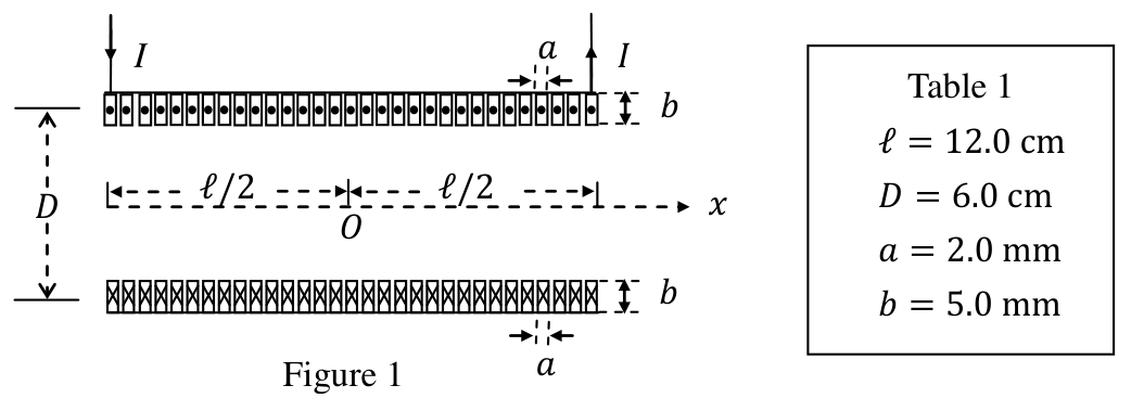
Figure 1

Table 1
$\ell =12.0$ cm
$D=6.0$ cm
$a=2.0$ mm
$b=5.0$ mm

In assessing if such a magnet can serve to provide high magnetic fields, two limiting factors must not be overlooked. One is the mechanical rigidity of the coil to withstand large Lorentz force on the field-producing current. The other is that the enormous amount of Joule heat generated in the wire must not cause excessive temperature rise. We shall examine these two factors using simplified models.

The Appendix at the end of the question lists some mathematical formulae and physical data which may be used if necessary.

Part A. Magnetic Fields on the Axis of the Coil

Assume $b\ll D$ so that one may regard the wire as a thin strip of width $a$. Let $O$ be the origin of $x$ coordinates. The direction of the current flow is as shown in Fig. 1.

(a) Find the $x$-component $B(x)$ of the magnetic field on the axis of the coil as a function of $x$ when the steady current passing through the coil is $I$. [1.0 point]

(b) Find the steady current $I_0$ passing through the coil if $B(0)$ is $10.0$ T. Use data given in Table 1 when computing numerical values. [0.4 point]

Part B. The Upper Limit of Current

In Part B, we assume the length $\ell$ of the coil is infinite and $b\ll D$. Consider the turn of the coil located at $x=0$. The magnetic field exerts Lorentz force on the current passing through the turn. Thus, as Fig. 2 shows, a wire segment of length $\Delta s$ is subject to a normal force $\Delta F_n$ which tends to make the turn expand.

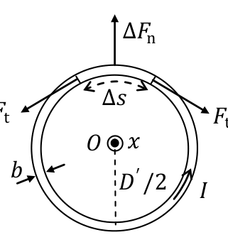
Figure 2

(c) Suppose that, when the current is $I$, the mean diameter of the expanded coil remains at a constant value $D^{\prime }$ larger than $D$, as shown in Fig. 2.

Find the outward normal force per unit length $\Delta F_n/\Delta s$. [1.2 point]

Find the tension $F_t$ acting along the wire. [0.6 point]

(d) Neglect the coil’s acceleration during the expansion. Assume the turn will break when the wire’s unit elongation (i.e. tensile strain or fractional change of the length) is 60 % and tensile stress (i.e. tension per unit cross sectional area of the unstrained wire) is ${\sigma }_b=455\mathrm{MPa}$. Let $I_b$ be the current at which the turn will break and $B_b$ the corresponding magnetic field at the center $O$.

Find an expression for $I_b$ and then calculate its value. [0.8 point]

Find an expression for $B_b$ and then calculate its value. [0.4 point]

Part C. The Rate of Temperature Rise

When the current $I$ is $10.0$ kA and the temperature $T$ of the coil is $293$ K, assume that the resistivity, the specific heat capacity at constant pressure, and the mass density of the wire of the coil are, respectively, given by ${\rho }_e=1.72\times 10^{-8}\Omega \cdot \mathrm{m}$, $c_p=3.85\times 10^{2}J/(\mathrm{kg}\cdot \mathrm{K})$ and ${\rho }_m=8.98\times 10^3\mathrm{kg}\cdot {\mathrm{m}}^{-3}$.

(e) Find an expression for the power density (i.e. power per unit volume) of heat generation in the coil and then calculate its value. Use data in Table 1. [0.5 point]

(f) Let $\dot{T}$ be the time rate of change of temperature in the coil. Find an expression for $\dot{T}$ and then calculate its value. [0.5 point]

Part D. A Pulsed-Field Magnet

If the large current needed for a strong magnet lasts only for a short time, the temperature rise caused by excessive Joule heating may be greatly reduced. This idea is employed in a pulsed-field magnet.

Thus, as shown in Fig. 3, a capacitor bank of capacitance $C$ charged initially to a potential $V_0$ is used to drive the current $I$ through the coil. The circuit is equipped with a switch $K$. The inductance $L$ and resistance $R$ of the circuit are assumed to be entirely due to the coil. The construct and dimensions of the coil are the same as given in Fig. 1 and Table 1. Assume $R$, $L$, and $C$ to be independent of temperature and the magnetic field is the same as that of an infinite solenoid with $\ell \to \infty$.

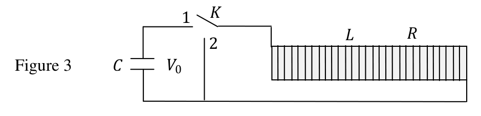
Figure 3

(g) Find expressions for the inductance $L$ and resistance $R$. [0.6 point]

Calculate the values of $L$ and $R$. Use data given in Table 1. [0.4 point]

(h) At time $t=0$, the switch $K$ is thrown to position 1 and the current starts flowing. For $t\ge 0$, the charge $Q(t)$ on the positive plate of the capacitor and the current $I(t)$ entering the positive plate are given by

Q(t) = \frac{CV_0}{\sin \theta_0} e^{-\alpha t} \sin(\omega t + \theta_0), \tag{1}

I(t) = \frac{dQ}{dt} = \left(\frac{-\alpha}{\cos \theta_0}\right) \frac{CV_0}{\sin \theta_0} e^{-\alpha t} \sin \omega t, \tag{2}

in which $\alpha$ and $\omega$ are positive constants and ${\theta }_0$ is given by

\tan \theta_0 = \frac{\omega}{\alpha}, \qquad 0 < \theta_0 < \frac{\pi}{2}. \tag{3}

Note that, if $Q(t)$ is expressed as a function of a new variable $t^{\prime }\equiv (t+{\theta }_0/\omega )$, then $Q(t^{\prime })$ and its time derivative $I(t)$ are identical in form except for an overall constant factor. The time derivative of $I(t)$ may therefore be obtained similarly without further differentiations.

Find $\alpha$ and $\omega$ in terms of $R$, $L$, and $C$. [0.8 point]

Calculate the values of $\alpha$ and $\omega$ when $C$ is $10.0$ mF. [0.4 point]

(i) Let $I_m$ be the maximum value of $|I(t)|$ for $t>0$. Find an expression for $I_m$. [0.6 point]

If $C=10.0$ mF, what is the maximum value $V_{0b}$ of the initial voltage $V_0$ of the capacitor bank for which $I_m$ will not exceed $I_b$ found in Problem (d)? [0.4 point]

(j) Suppose the switch $K$ is moved instantly from position 1 to 2 when the absolute value of the current $|I(t)|$ reaches $I_m$. Let $\Delta E$ be the total amount of heat dissipated in the coil from $t=0$ to $\infty$ and $\Delta T$ the corresponding temperature increase of the coil. Assume the initial voltage $V_0$ takes on the maximum value $V_{0b}$ obtained in Problem (i) and the electromagnetic energy loss is only in the form of heat dissipated in the coil.

Find an expression for $\Delta E$ and then calculate its value. [1.0 point]

Find an expression for $\Delta T$ and then calculate its value. Note that the value for $\Delta T$ must be compatible with the assumption of constant $R$ and $L$. [0.4 point]

Appendix

1. ${\int }_0^L\frac{dx}{(D^2+x^2{)}^{3/2}}=\frac{1}{D^2}\left\{\frac{L}{(D^2+L^2{)}^{1/2}}\right\}$

2. $\sin (\alpha \pm \beta )=\sin \alpha \cos \beta \pm \cos \alpha \sin \beta$

3. permeability of free space ${\mu }_0=4\pi \times 10^{-7}\mathrm{T}\cdot m/A$

Fonte: Testo (PDF) — p.1

Topic: Electromagnetism, Circuits, Elasticity & Materials Metodi: Biot-Savart Law, Lorentz Force Analysis, Stress-Strain Analysis, Differential Equations Competenze: Mathematical Modeling, Physical Reasoning, Unit Conversion Objects: Solenoid, Wire, Capacitor, Switch

Domanda teorica 2 Forti elettromagneti resistenti

L’elettromagneto resistente è un magneto con bobine di un metallo normale come il rame o l’alluminio. I moderni elettromagneti resistenti forti possono fornire campi magnetici stabili superiori a 30 tesla. Le loro bobine sono tipicamente costruite impiandando centinaia di sottili lastre circolari di lamiera di rame con molti buchi di raffreddamento stampati in esse; ci sono anche isolanti con lo stesso schema. Quando si applica una tensione attraverso la bobina, la corrente scorre attraverso le piastre lungo un percorso elicico per generare alti campi magnetici nel centro del magnete.

In questa domanda si intende valutare se una bobina cilindrica (o solenoide) di molte giri può servire da magnete per generare campi magnetici elevati. Come mostrato nella figura. 1, il centro del magnete è a $O$. La sua bobina cilindrica è costituita da giri $N$ di filo di rame con corrente $I$ uniformemente distribuita sulla sezione trasversale del filo. Il diametro medio della bobina è $D$ e la sua lunghezza lungo la direzione asiale $x$ è $\ell$. La sezione trasversale del filo è rettangolare, con larghezza $a$ e altezza $b$. Le curve della bobina sono così strettamente rotte che il piano di ciascuna curva può essere considerato perpendicolare all’asse $x$ e $\ell =Nb$. Nella tabella 1 sono elencati i dati specifici delle dimensioni fisiche della bobina.

Figura 1

∙ ∙ Tavola 1 ∙
$\ell =12.0$ cm
$D=6.0$ cm
$a=2.0$ mm
$b=5.0$ mm

Nel valutare se un tale magnete possa servire a fornire campi magnetici elevati, non si devono trascurare due fattori limitanti. Uno è la rigidità meccanica della bobina per resistere a una grande forza di Lorentz sulla corrente prodotta nel campo. L’altro è che l’enorme quantità di calore Joule generato nel filo non deve causare un aumento eccessivo della temperatura. Esamineremo questi due fattori utilizzando modelli semplificati.

L’appendice alla fine della domanda elenca alcune formule matematiche e dati fisici che possono essere utilizzati se necessario.

Parte A. Campo magnetico sull’asse della bobina

Supponiamo $b\ll D$ in modo da considerare il filo come una sottile striscia di larghezza $a$. La fonte delle coordinate $x$ è $O$. La direzione del flusso corrente è mostrata nella figura. 1.

**(a) ** Trova la componente $x$ $B(x)$ del campo magnetico sull’asse della bobina come funzione di $x$ quando la corrente costante che attraversa la bobina è $I$. [1,0 punto]

**(b) ** Trova la corrente fissa $I_0$ che passa attraverso la bobina se $B(0)$ è $10.0$ T. Utilizzare i dati di cui alla tabella 1 per calcolare i valori numerici. [0,4 punto]

Parte B. Il limite superiore della corrente

Nella parte B, supponiamo che la lunghezza $\ell$ della bobina sia infinita e $b\ll D$. Considerare la rotazione della bobina situata a $x=0$. Il campo magnetico esercita la forza di Lorentz sulla corrente che passa attraverso la curva. Così, come Fig. 2 indica che un segmento di filo di lunghezza $\Delta s$ è soggetto a una forza normale $\Delta F_n$ che tende a far espandere la curva.

Figura 2

**(c) ** Supponiamo che, quando la corrente è $I$, il diametro medio della bobina ampliata rimanga a un valore costante $D^{\prime }$ maggiore di $D$, come mostrato nella figura. 2.

Trova la forza normale esterna per lunghezza unitaria $\Delta F_n/\Delta s$. [1,2 punto]

Trova la tensione $F_t$ che agisce lungo il filo. [0,6 punto]

**(d) ** Trascurare l’accelerazione della bobina durante l’espansione. Supponiamo che la curva si rompa quando l’allungamento unitario del filo (cioè tensione di trazione o variazione frazionaria della lunghezza) è del 60% e tensione di trazione (cioè tensione per unità di superficie trasversale del filo non tenso) è ${\sigma }_b=455\mathrm{MPa}$. Let $I_b$ be the current at which the turn will break and $B_b$ the corresponding magnetic field at the center $O$.

Trova un’espressione per $I_b$ e quindi calcola il suo valore. [0,8 punto]

Trova un’espressione per $B_b$ e quindi calcola il suo valore. [0,4 punto]

Parte C. Il tasso di aumento della temperatura

Quando la corrente $I$ è $10.0$ kA e la temperatura $T$ della bobina è $293$ K, supponiamo che la resistività, la capacità termica specifica a pressione costante e la densità di massa del filo della bobina siano, rispettivamente, dati da ${\rho }_e=1.72\times 10^{-8}\Omega \cdot \mathrm{m}$, $c_p=3.85\times 10^{2}J/(\mathrm{kg}\cdot \mathrm{K})$ e ${\rho }_m=8.98\times 10^3\mathrm{kg}\cdot {\mathrm{m}}^{-3}$.

**(e) ** Trova un’espressione per la densità di potenza ** (cioè potenza per unità di volume) della produzione di calore nella bobina e quindi calcolare il suo valore. Utilizzare i dati riportati nella tabella 1. [0,5 punto]

**(f) ** $\dot{T}$ deve essere il tasso temporale di variazione della temperatura della bobina. Trova un’espressione per $\dot{T}$ e quindi calcola il suo valore. [0,5 punto]

Parte D. Un magnete a campo pulsato

Se la corrente elevata necessaria per un magnete forte dura solo per un breve periodo, l’aumento della temperatura causato da un eccessivo riscaldamento Joule può essere notevolmente ridotto. Questa idea è impiegata in un magnete a campo pulsato **.

Così, come si vede in Figura 1. 3, per guidare la corrente $I$ attraverso la bobina viene utilizzata una banca di condensatori di capacità $C$ caricata inizialmente a un potenziale $V_0$. Il circuito è dotato di un interruttore $K$. Si presume che l’induttanza $L$ e la resistenza $R$ del circuito siano interamente dovute alla bobina. La struttura e le dimensioni della bobina sono le stesse di quelle riportate nella figura. 1 e tabella 1. Supponiamo che $R$, $L$ e $C$ siano indipendenti dalla temperatura e che il campo magnetico sia lo stesso di un solenoide infinito con $\ell \to \infty$.

Figura 3

**(g) ** Trova espressioni per l’induzione $L$ e la resistenza $R$. [0,6 punto]

Calcolare i valori di $L$ e $R$. Utilizzare i dati riportati nella tabella 1. [0,4 punto]

**(h) ** Al momento $t=0$, il interruttore $K$ viene gettato alla posizione 1 e la corrente inizia a fluire. Per $t\ge 0$, la carica $Q(t)$ sulla piastra positiva del condensatore e la corrente $I(t)$ che entra nella piastra positiva sono indicate da:

Q(t) = \frac{CV_0}{\sin \theta_0} e^{-\alpha t} \sin(\omega t + \theta_0), \tag{1}

I(t) = \frac{dQ}{dt} = \left(\frac{-\alpha}{\cos \theta_0}\right) \frac{CV_0}{\sin \theta_0} e^{-\alpha t} \sin \omega t, \tag{2}

in cui $\alpha$ e $\omega$ sono costanti positive e ${\theta }_0$ è dato da

\tan \theta_0 = \frac{\omega}{\alpha}, \qquad 0 < \theta_0 < \frac{\pi}{2}. \tag{3}

Si noti che, se $Q(t)$ è espressa come funzione di una nuova variabile $t^{\prime }\equiv (t+{\theta }_0/\omega )$, allora $Q(t^{\prime })$ e la sua derivata temporale $I(t)$ sono identici nella forma, tranne per un fattore costante complessivo. La derivata temporale di $I(t)$ può quindi essere ottenuta in modo simile senza ulteriori differenziazioni.

Trova $\alpha$ e $\omega$ in termini di $R$, $L$ e $C$. [0,8 punto]

Calcolare i valori di $\alpha$ e $\omega$ quando $C$ è $10.0$ mF. [0,4 punto]

**(i) ** $I_m$ deve essere il valore massimo di $|I(t)|$ per $t>0$. Trova un’espressione per $I_m$. [0,6 punto]

Se $C=10.0$ mF, qual è il valore massimo $V_{0b}$ della tensione iniziale $V_0$ della banca condensatore per la quale $I_m$ non supererà $I_b$ riscontrato nel problema (d)? [0,4 punto]

**(j) ** Supponiamo che il switch $K$ sia spostato istantaneamente dalla posizione 1 alla posizione 2 quando il valore assoluto della corrente $|I(t)|$ raggiunge $I_m$. Il $\Delta E$ è la quantità totale di calore dissipato nella bobina da $t=0$ a $\infty$ e $\Delta T$ l’aumento di temperatura corrispondente della bobina. Supponiamo che la tensione iniziale $V_0$ assume il valore massimo $V_{0b}$ ottenuto nel problema (i) e che la perdita di energia elettromagnetica sia solo sotto forma di calore dissipato nella bobina.

Trova un’espressione per $\Delta E$ e quindi calcola il suo valore. [1,0 punto]

Trova un’espressione per $\Delta T$ e quindi calcola il suo valore. Si noti che il valore di $\Delta T$ deve essere compatibile con l’ipotesi di costanti $R$ e $L$. [0,4 punto]

Appendice

1. ${\int }_0^L\frac{dx}{(D^2+x^2{)}^{3/2}}=\frac{1}{D^2}\left\{\frac{L}{(D^2+L^2{)}^{1/2}}\right\}$

2. $\sin (\alpha \pm \beta )=\sin \alpha \cos \beta \pm \cos \alpha \sin \beta$

3. permeabilità dello spazio libero ${\mu }_0=4\pi \times 10^{-7}\mathrm{T}\cdot m/A$

Fonte: Testo (PDF) — p.1

Topic: Electromagnetism, Circuits, Elasticity & Materials Metodi: Biot-Savart Law, Lorentz Force Analysis, Stress-Strain Analysis, Differential Equations Competenze: Mathematical Modeling, Physical Reasoning, Unit Conversion Objects: Solenoid, Wire, Capacitor, Switch

Theoretical Question 3 — Electron and Gas Bubbles in Liquids

This question deals with physics of two bubble-in-liquid systems. It has two parts:

• Part A. An electron bubble in liquid helium
• Part B. Single gas bubble in liquid

Part A. An Electron Bubble in Liquid Helium

When an electron is planted inside liquid helium, it can repel atoms of liquid helium and form what is called an electron bubble. The bubble contains nothing but the electron itself. We shall be interested mainly in its size and stability.

We use $\Delta f$ to denote the uncertainty of a quantity $f$. The components of an electron’s position vector $\vec{q}=(x,y,z)$ and momentum vector $\vec{p}=(p_x,p_y,p_z)$ must obey Heisenberg’s uncertainty relations $\Delta q_{\alpha }\Delta p_{\alpha }\ge \hslash /2$, where $\hslash$ is the Planck constant divided by $2\pi$ and $\alpha =x,y,z$.

We shall assume the electron bubble to be isotropic and its interface with liquid helium is a sharp spherical surface. The liquid is kept at a constant temperature very close to $0$ K with its surface tension $\sigma$ given by $3.75\times 10^{-4}\mathrm{N}\cdot {\mathrm{m}}^{-1}$ and its electrostatic responses to the electron bubble may be neglected.

Consider an electron bubble in liquid helium with an equilibrium radius $R$. The electron, of mass $m$, moves freely inside the bubble with kinetic energy $E_k$ and exerts pressure $P_e$ on the inner side of the bubble-liquid interface. The pressure exerted by liquid helium on the outer side of the interface is $P_{He}$.

(a) Find a relation between $P_{He}$, $P_e$, and $\sigma$. [0.4 point]

Find a relation between $E_k$ and $P_e$. [1.0 point]

(b) Denote by $E_0$ the smallest possible value of $E_k$ consistent with Heisenberg’s uncertainty relations when the electron is inside the bubble of radius $R$. Estimate $E_0$ as a function of $R$. [0.8 point]

(c) Let $R_e$ be the equilibrium radius of the bubble when $E_k=E_0$ and $P_{He}=0$.

Obtain an expression for $R_e$ and calculate its value. [0.6 point]

(d) Find a condition that $R$ and $P_{He}$ must satisfy if the equilibrium at radius $R$ is to be locally stable under constant $P_{He}$. Note that $P_{He}$ can be negative. [0.6 point]

(e) There exists a threshold pressure $P_{th}$ such that equilibrium is not possible for the electron bubble when $P_{He}$ is less than $P_{th}$. Find an expression for $P_{th}$. [0.6 point]

Part B. Single Gas Bubble in Liquid — Collapsing and Radiation

In this part of the problem, we consider a normal liquid, such as water.

When a gas bubble in a liquid is driven by an oscillating pressure, it can show dramatic responses. For example, following a large expansion, it can collapse rapidly to a small radius and, near the end of the collapse, emit light almost instantly. In this phenomenon, called single-bubble sonoluminescence, the gas bubble undergoes cyclic motions which typically consist of three stages: expansion, collapse, and multiple after-bounces. In the following we shall focus mainly on the collapsing stage.

We assume that, at all times, the bubble considered is spherical and its center remains stationary in the liquid. See Fig 1. The pressure, temperature, and density are always uniform inside the bubble as its size diminishes. The liquid containing the bubble is assumed to be isotropic, nonviscous, incompressible, and very much larger in extent than the bubble. All effects due to gravity and surface tension are neglected so that pressures on both sides of the bubble-liquid interface are always equal.

Radial motion of the bubble-liquid interface

As the bubble’s radius $R=R(t)$ changes with time $t$, the bubble-liquid interface will move with radial velocity $\dot{R}\equiv dR/dt$. It follows from the equation of continuity of incompressible fluids that the liquid’s radial velocity $\dot{r}\equiv dr/dt$ at distance $r$ from the center of the bubble is related to the rate of change of the bubble’s volume $V$ by

\frac{dV}{dt} = 4\pi R^2 \dot{R} = 4\pi r^2 \dot{r}. \tag{1}

This implies that the total kinetic energy $E_k$ of the liquid with mass density ${\rho }_0$ is

E_k = \frac{1}{2} \int_R^{r_0} \rho_0 (4\pi r^2 dr)\dot{r}^2 = 2\pi \rho_0 R^4 \dot{R}^2 \int_R^{r_0} \frac{1}{r^2} dr = 2\pi \rho_0 R^4 \dot{R}^2 \left(\frac{1}{R} - \frac{1}{r_0}\right) \tag{2}

where $r_0$ is the radius of the outer surface of the liquid.

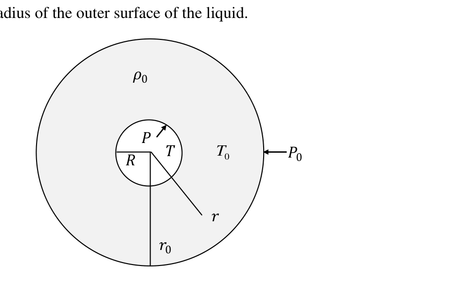
Fig. 1

(f) Assume the ambient pressure $P_0$ acting on the outer surface $r=r_0$ of the liquid is constant. Let $P=P(R)$ be the gas pressure when the radius of the bubble is $R$.

Find the amount of work $dW$ done on the liquid when the radius of the bubble changes from $R$ to $R+dR$. Use $P_0$ and $P$ to express $dW$. [0.4 point]

The work $dW$ must be equal to the corresponding change in the total kinetic energy of the liquid. In the limit $r_0\to \infty$, it follows that we have Bernoulli’s equation in the form

\frac{1}{2} \rho_0 \, d\!\left(R^m \dot{R}^2\right) = (P - P_0)R^n dR. \tag{3}

Find the exponents $m$ and $n$ in Eq. (3). Use dimensional arguments if necessary. [0.4 point]

Collapsing of the gas bubble

From here on, we consider only the collapsing stage of the bubble. The mass density of the liquid is ${\rho }_0=1.0\times 10^3\mathrm{kg}\cdot {\mathrm{m}}^{-3}$, the temperature $T_0$ of the liquid is $300$ K and the ambient pressure $P_0$ is $1.01\times 10^5\mathrm{Pa}$. We assume that ${\rho }_0$, $T_0$, and $P_0$ remain constant at all times and the bubble collapses adiabatically without any exchange of mass across the bubble-liquid interface.

The bubble considered is filled with an ideal gas. The ratio of specific heat at constant pressure to that at constant volume for the gas is $\gamma =5/3$. When under temperature $T_0$ and pressure $P_0$, the equilibrium radius of the bubble is $R_0=5.00\mu \mathrm{m}$.

Now, this bubble begins its collapsing stage at time $t=0$ with $R(0)=R_i=7R_0$, $\dot{R}(0)=0$, and the gas temperature $T_i=T_0$. Note that, because of the bubble’s expansion in the preceding stage, $R_i$ is considerably larger than $R_0$ and this is necessary if sonoluminescence is to occur.

(g) Express the pressure $P\equiv P(R)$ and temperature $T\equiv T(R)$ of the ideal gas in the bubble as a function of $R$ during the collapsing stage, assuming quasi-equilibrium conditions hold. [0.6 point]

(h) Let $\beta \equiv R/R_i$ and $\dot{\beta }=d\beta /dt$. Eq. (3) implies a conservation law which takes the following form

\frac{1}{2} \rho_0 \dot{\beta}^2 + U(\beta) = 0. \tag{4}

Let $P_i\equiv P(R_i)$ be the gas pressure of the bubble when $R=R_i$. If we introduce the ratio $Q\equiv P_i/[(\gamma -1)P_0]$, the function $U(\beta )$ may be expressed as

U(\beta) = \mu \beta^{-5}\left[Q(1 - \beta^2) - \beta^2(1 - \beta^3)\right]. \tag{5}

Find the coefficient $\mu$ in terms of $R_i$ and $P_0$. [0.6 point]

(i) Let $R_m$ be the minimum radius of the bubble during the collapsing stage and define ${\beta }_m\equiv R_m/R_i$. For $Q\ll 1$, we have ${\beta }_m\approx C_m\sqrt{Q}$.

Find the constant $C_m$. [0.4 point]

Evaluate $R_m$ for $R_i=7R_0$. [0.3 point]

Evaluate the temperature $T_m$ of the gas at $\beta ={\beta }_m$. [0.3 point]

(j) Assume $R_i=7R_0$. Let ${\beta }_u$ be the value of $\beta$ at which the dimensionless radial speed $u\equiv |\dot{\beta }|$ reaches its maximum value. The gas temperature rises rapidly for values of $\beta$ near ${\beta }_u$.

Give an expression and then estimate the value of ${\beta }_u$. [0.6 point]

Let $\bar{u}$ be the value of $u$ at $\beta =\bar{\beta }\equiv ({\beta }_m+{\beta }_u)/2$. Evaluate $\bar{u}$. [0.4 point]

Give an expression and then estimate the duration $\Delta t_m$ of time needed for $\beta$ to diminish from ${\beta }_u$ to the minimum value ${\beta }_m$. [0.6 point]

Sonoluminescence of the collapsing bubble

Consider the bubble to be a surface black-body radiator of constant emissivity $a$ so that the effective Stefan-Boltzmann’s constant ${\sigma }_{\mathrm{eff}}=a{\sigma }_{SB}$. If the collapsing stage is to be approximated as adiabatic, the emissivity must be small enough so that the power radiated by the bubble at $\beta =\bar{\beta }$ is no more than a fraction, say 20 %, of the power $\dot{E}$ supplied to it by the driving liquid pressure.

(k) Find the power $\dot{E}$ supplied to the bubble as a function of $\beta$. [0.6 point]

Give an expression and then estimate the value for an upper bound of $a$. [0.8 point]

Appendix

1. $\frac{d}{dx}{x}^n=n{x}^{n-1}$

2. Electron mass $m=9.11\times 10^{-31}\mathrm{kg}$

3. Planck constant $h=2\pi \hslash =2\pi \times 1.055\times 10^{-34}\mathrm{J}\cdot \mathrm{s}$

4. Stefan-Boltzmann’s constant ${\sigma }_{SB}=5.67\times 10^{-8}\mathrm{W}\cdot {\mathrm{m}}^{-2}\cdot {\mathrm{K}}^{-4}$

Fonte: Testo (PDF) — p.1

Topic: Fluid Mechanics, Modern-Quantum Physics, Thermodynamics Metodi: Bernoulli’s Equation, Continuity Equation, Energy Conservation Method, Calculus-Integration Competenze: Mathematical Modeling, Physical Reasoning, Estimation & Approximation Objects: Bubble, Electron, Gas

Domanda Teorica 3 — Bolle di elettrone e di gas nei liquidi

Questa domanda tratta la fisica di due sistemi bolla-in-liquido. È composta da due parti:

• Parte A. Una bolla di elettrone nell’elio liquido
• Parte B. Singola bolla di gas in un liquido

Parte A. Una bolla di elettrone nell’elio liquido

Quando un elettrone viene collocato all’interno dell’elio liquido, può respingere gli atomi di elio liquido e formare ciò che si chiama bolla di elettrone. La bolla non contiene nient’altro che l’elettrone stesso. Ci interesseremo principalmente della sua dimensione e della sua stabilità.

Usiamo $\Delta f$ per indicare l’incertezza di una grandezza $f$. Le componenti del vettore posizione $\vec{q}=(x,y,z)$ e del vettore quantità di moto $\vec{p}=(p_x,p_y,p_z)$ di un elettrone devono obbedire alle relazioni di indeterminazione di Heisenberg $\Delta q_{\alpha }\Delta p_{\alpha }\ge \hslash /2$, dove $\hslash$ è la costante di Planck divisa per $2\pi$ e $\alpha =x,y,z$.

Assumeremo che la bolla di elettrone sia isotropa e che la sua interfaccia con l’elio liquido sia una superficie sferica netta. Il liquido è mantenuto a una temperatura costante molto vicina a $0$ K con tensione superficiale $\sigma$ data da $3.75\times 10^{-4}\mathrm{N}\cdot {\mathrm{m}}^{-1}$ e le sue risposte elettrostatiche alla bolla di elettrone possono essere trascurate.

Considera una bolla di elettrone nell’elio liquido con raggio di equilibrio $R$. L’elettrone, di massa $m$, si muove liberamente all’interno della bolla con energia cinetica $E_k$ ed esercita una pressione $P_e$ sul lato interno dell’interfaccia bolla-liquido. La pressione esercitata dall’elio liquido sul lato esterno dell’interfaccia è $P_{He}$.

(a) Trova una relazione tra $P_{He}$, $P_e$ e $\sigma$. [0.4 punti]

Trova una relazione tra $E_k$ e $P_e$. [1.0 punti]

(b) Indica con $E_0$ il più piccolo valore possibile di $E_k$ compatibile con le relazioni di indeterminazione di Heisenberg quando l’elettrone si trova all’interno della bolla di raggio $R$. Stima $E_0$ in funzione di $R$. [0.8 punti]

(c) Sia $R_e$ il raggio di equilibrio della bolla quando $E_k=E_0$ e $P_{He}=0$.

Ricava un’espressione per $R_e$ e calcolane il valore. [0.6 punti]

(d) Trova una condizione che $R$ e $P_{He}$ devono soddisfare affinché l’equilibrio al raggio $R$ sia localmente stabile a $P_{He}$ costante. Nota che $P_{He}$ può essere negativa. [0.6 punti]

(e) Esiste una pressione di soglia $P_{th}$ tale che l’equilibrio non è possibile per la bolla di elettrone quando $P_{He}$ è minore di $P_{th}$. Trova un’espressione per $P_{th}$. [0.6 punti]

Parte B. Singola bolla di gas in un liquido — Collasso e radiazione

In questa parte del problema, consideriamo un liquido normale, come l’acqua.

Quando una bolla di gas in un liquido è pilotata da una pressione oscillante, può mostrare risposte spettacolari. Per esempio, in seguito a una grande espansione, può collassare rapidamente fino a un raggio piccolo e, verso la fine del collasso, emettere luce quasi istantaneamente. In questo fenomeno, chiamato sonoluminescenza a bolla singola, la bolla di gas subisce moti ciclici che tipicamente consistono di tre stadi: espansione, collasso e molteplici rimbalzi successivi. Nel seguito ci concentreremo principalmente sullo stadio di collasso.

Assumiamo che, in ogni istante, la bolla considerata sia sferica e che il suo centro rimanga fermo nel liquido. Vedi Fig 1. La pressione, la temperatura e la densità sono sempre uniformi all’interno della bolla man mano che la sua dimensione diminuisce. Il liquido che contiene la bolla è assunto isotropo, non viscoso, incomprimibile e di estensione molto maggiore della bolla. Tutti gli effetti dovuti alla gravità e alla tensione superficiale sono trascurati, così che le pressioni sui due lati dell’interfaccia bolla-liquido sono sempre uguali.

Moto radiale dell’interfaccia bolla-liquido

Poiché il raggio della bolla $R=R(t)$ varia nel tempo $t$, l’interfaccia bolla-liquido si muoverà con velocità radiale $\dot{R}\equiv dR/dt$. Dall’equazione di continuità dei fluidi incomprimibili segue che la velocità radiale del liquido $\dot{r}\equiv dr/dt$ a distanza $r$ dal centro della bolla è legata al tasso di variazione del volume della bolla $V$ da

\frac{dV}{dt} = 4\pi R^2 \dot{R} = 4\pi r^2 \dot{r}. \tag{1}

Ciò implica che l’energia cinetica totale $E_k$ del liquido di densità di massa ${\rho }_0$ è

E_k = \frac{1}{2} \int_R^{r_0} \rho_0 (4\pi r^2 dr)\dot{r}^2 = 2\pi \rho_0 R^4 \dot{R}^2 \int_R^{r_0} \frac{1}{r^2} dr = 2\pi \rho_0 R^4 \dot{R}^2 \left(\frac{1}{R} - \frac{1}{r_0}\right) \tag{2}

dove $r_0$ è il raggio della superficie esterna del liquido.

Fig. 1

(f) Assumi che la pressione ambiente $P_0$ che agisce sulla superficie esterna $r=r_0$ del liquido sia costante. Sia $P=P(R)$ la pressione del gas quando il raggio della bolla è $R$.

Trova la quantità di lavoro $dW$ compiuto sul liquido quando il raggio della bolla varia da $R$ a $R+dR$. Usa $P_0$ e $P$ per esprimere $dW$. [0.4 punti]

Il lavoro $dW$ deve essere uguale alla corrispondente variazione dell’energia cinetica totale del liquido. Nel limite $r_0\to \infty$, segue che si ha l’equazione di Bernoulli nella forma

\frac{1}{2} \rho_0 \, d\!\left(R^m \dot{R}^2\right) = (P - P_0)R^n dR. \tag{3}

Trova gli esponenti $m$ e $n$ nell’Eq. (3). Usa argomenti dimensionali se necessario. [0.4 punti]

Collasso della bolla di gas

Da qui in poi, consideriamo solo lo stadio di collasso della bolla. La densità di massa del liquido è ${\rho }_0=1.0\times 10^3\mathrm{kg}\cdot {\mathrm{m}}^{-3}$, la temperatura $T_0$ del liquido è $300$ K e la pressione ambiente $P_0$ è $1.01\times 10^5\mathrm{Pa}$. Assumiamo che ${\rho }_0$, $T_0$ e $P_0$ rimangano costanti in ogni istante e che la bolla collassi adiabaticamente senza alcuno scambio di massa attraverso l’interfaccia bolla-liquido.

La bolla considerata è riempita con un gas ideale. Il rapporto tra il calore specifico a pressione costante e quello a volume costante per il gas è $\gamma =5/3$. Alla temperatura $T_0$ e pressione $P_0$, il raggio di equilibrio della bolla è $R_0=5.00\mu \mathrm{m}$.

Ora, questa bolla inizia il suo stadio di collasso al tempo $t=0$ con $R(0)=R_i=7R_0$, $\dot{R}(0)=0$, e temperatura del gas $T_i=T_0$. Nota che, a causa dell’espansione della bolla nello stadio precedente, $R_i$ è considerevolmente maggiore di $R_0$ e ciò è necessario affinché avvenga la sonoluminescenza.

(g) Esprimi la pressione $P\equiv P(R)$ e la temperatura $T\equiv T(R)$ del gas ideale nella bolla in funzione di $R$ durante lo stadio di collasso, assumendo che valgano condizioni di quasi-equilibrio. [0.6 punti]

(h) Sia $\beta \equiv R/R_i$ e $\dot{\beta }=d\beta /dt$. L’Eq. (3) implica una legge di conservazione che assume la forma seguente

\frac{1}{2} \rho_0 \dot{\beta}^2 + U(\beta) = 0. \tag{4}

Sia $P_i\equiv P(R_i)$ la pressione del gas della bolla quando $R=R_i$. Se introduciamo il rapporto $Q\equiv P_i/[(\gamma -1)P_0]$, la funzione $U(\beta )$ può essere espressa come

U(\beta) = \mu \beta^{-5}\left[Q(1 - \beta^2) - \beta^2(1 - \beta^3)\right]. \tag{5}

Trova il coefficiente $\mu$ in termini di $R_i$ e $P_0$. [0.6 punti]

(i) Sia $R_m$ il raggio minimo della bolla durante lo stadio di collasso e definisci ${\beta }_m\equiv R_m/R_i$. Per $Q\ll 1$, si ha ${\beta }_m\approx C_m\sqrt{Q}$.

Trova la costante $C_m$. [0.4 punti]

Valuta $R_m$ per $R_i=7R_0$. [0.3 punti]

Valuta la temperatura $T_m$ del gas a $\beta ={\beta }_m$. [0.3 punti]

(j) Assumi $R_i=7R_0$. Sia ${\beta }_u$ il valore di $\beta$ al quale la velocità radiale adimensionale $u\equiv |\dot{\beta }|$ raggiunge il suo valore massimo. La temperatura del gas sale rapidamente per valori di $\beta$ vicini a ${\beta }_u$.

Fornisci un’espressione e poi stima il valore di ${\beta }_u$. [0.6 punti]

Sia $\bar{u}$ il valore di $u$ a $\beta =\bar{\beta }\equiv ({\beta }_m+{\beta }_u)/2$. Valuta $\bar{u}$. [0.4 punti]

Fornisci un’espressione e poi stima la durata $\Delta t_m$ del tempo necessario affinché $\beta$ diminuisca da ${\beta }_u$ al valore minimo ${\beta }_m$. [0.6 punti]

Sonoluminescenza della bolla che collassa

Considera la bolla come un radiatore superficiale di corpo nero di emissività costante $a$, così che la costante efficace di Stefan-Boltzmann sia ${\sigma }_{\mathrm{eff}}=a{\sigma }_{SB}$. Se lo stadio di collasso deve essere approssimato come adiabatico, l’emissività deve essere abbastanza piccola così che la potenza irradiata dalla bolla a $\beta =\bar{\beta }$ non sia superiore a una frazione, diciamo il 20 %, della potenza $\dot{E}$ fornitale dalla pressione del liquido pilotante.

(k) Trova la potenza $\dot{E}$ fornita alla bolla in funzione di $\beta$. [0.6 punti]

Fornisci un’espressione e poi stima il valore di un limite superiore per $a$. [0.8 punti]

Appendice

1. $\frac{d}{dx}{x}^n=n{x}^{n-1}$

2. Massa dell’elettrone $m=9.11\times 10^{-31}\mathrm{kg}$

3. Costante di Planck $h=2\pi \hslash =2\pi \times 1.055\times 10^{-34}\mathrm{J}\cdot \mathrm{s}$

4. Costante di Stefan-Boltzmann ${\sigma }_{SB}=5.67\times 10^{-8}\mathrm{W}\cdot {\mathrm{m}}^{-2}\cdot {\mathrm{K}}^{-4}$

Fonte: Testo (PDF) — p.1

Topic: Fluid Mechanics, Modern-Quantum Physics, Thermodynamics Metodi: Bernoulli’s Equation, Continuity Equation, Energy Conservation Method, Calculus-Integration Competenze: Mathematical Modeling, Physical Reasoning, Estimation & Approximation Objects: Bubble, Electron, Gas