APhO 2011 — Sperimentale

Experimental Question 1: Levitation of Conductors in an Oscillating Magnetic Field

In an oscillating magnetic field of sufficient strength, levitation of a metal conductor becomes possible. The levitation occurs due to a non-zero mean magnetic force exerted on currents in the conductor. The currents are induced by the alternating field itself. The Lorentz force doesn’t average to zero because of a phase shift between the current oscillations and the magnetic field oscillations. This phase shift is a result of the self-inductance of the current loops within the conductor.

In this experiment, we study this phenomenon and deduce the self-inductance of an aluminum ring from measuring the vertical force applied to it by a solenoid with an oscillating current. For measurement convenience, the mean force on the ring will be directed downwards, so levitation will not be observed.

On your desk, you have the following items (Figure 1):

1. An AC power supply operating on 50 Hz. The power supply has two pairs of terminals. The two smaller sockets (1a) supply a voltage of about 24 V; use these only for running current through the solenoid. The two larger sockets (1b) supply a voltage of about 0.7 V. The power supply is turned on only when the green button (1c) is pressed — this is in order to prevent overheating the system by accidentally leaving the current on, as further explained below. The red light bulb indicates when the power supply is on.

2. A cylindrically symmetric solenoid filled with iron rods. The solenoid is connected to the 24 V terminals of the power supply. The solenoid can be raised and lowered using a long screw. The screw’s vertical step is $h=1.41\text{mm}$.

3.–5. Three metal rings made of exactly the same material (an alloy of aluminum). One ring is closed. The second ring is identical to the first except for a short segment which was removed, making the ring open. The third ring is also open, and is much thinner than the first two.

6.–7. Two multimeters. They will be used as a voltmeter and an ammeter. The AC voltmeter’s sensitivity is 0.1 mV. The ammeter can measure currents of up to 20 A (also in AC mode). Note: in AC mode, the multimeters display the RMS (root-mean-square) of the measured quantity, i.e. the amplitude divided by $\sqrt{2}$. See Figures 3 and 4 for detailed instructions.

8. A battery-powered digital scale with sensitivity 0.01 g. When the scale experiences a rapidly oscillating force, it displays the time-averaged force. Note: the scale has a “tare” option, which calibrates its reading under a given weight to zero. See Figure 2.

9. An $8\text{cm}\times 7\text{cm}\times 7\text{cm}$ polystyrene block which can be used as a stand for the rings.

10. Electric wires with various connectors.

11. A ruler.

12. Millimeter graph paper.

13. A desktop lamp which can be turned on or off for your convenience.

Caution: when the closed ring is exposed to the solenoid’s magnetic field, a large current flows through it, heating it up. As a consequence, the ring’s electrical properties may change slightly. To avoid this, don’t run a current through the solenoid for long periods of time.

The earth’s gravity field in Tel Aviv is $g=9.80\pm 0.01\text{N/kg}$.

Figure 1 — Summary of the equipment

(1) 50 Hz power supply; (1a) 24 V terminals; (1b) 0.7 V terminals; (1c) Power button. (2) Solenoid on a vertical screw. (3) Broad closed ring. (4) Broad open ring. (5) Thin open ring. (6) Voltmeter. (7) Ammeter. (8) Scale. (9) Polystyrene block. (10) Wires.

Figure 2 — The digital scale

(1) On/Off button. (2) “Tare” button — sets the current weight as 0.

Figure 3 — The voltmeter

(1) On/Off button. (2) The dial is set to 200 mV AC. (3) Connect your wires to the “COM” and “V/Ω” terminals.

Figure 4 — The ammeter

(1) On/Off button. (2) The dial is set to 20 mA / 20 A AC. (3) Connect your wires to the “COM” and “A” terminals.

Theory (1.3 points)

Consider a conducting ring of radius $r$ placed in the solenoid’s magnetic field. The symmetry axes of the solenoid and the ring coincide. Denote the ring’s inductance by $L$, its resistance by $R$, and the angular frequency of the solenoid’s current by $\omega$. Define $z$ as the coordinate along the common symmetry axis of the solenoid and the ring.

In this part only, you may neglect the small effect of the ring’s magnetic field on the solenoid and the iron. Also, neglect the thickness of the ring.

In this part, we’ll use Faraday’s law, and the magnetic version of Gauss’s law:

• Faraday’s law: The induced EMF (electromotive force) on a loop generated by a changing magnetic flux is $ϵ=-d{\Phi }_{\mathrm{B}}/dt$.
• The magnetic Gauss law: the total magnetic flux through a closed surface is zero.

A current loop placed in a cylindrically symmetric magnetic field $\vec{B}$ experiences a total force

$F(t)=-2\pi rI(t)B_r(t)$

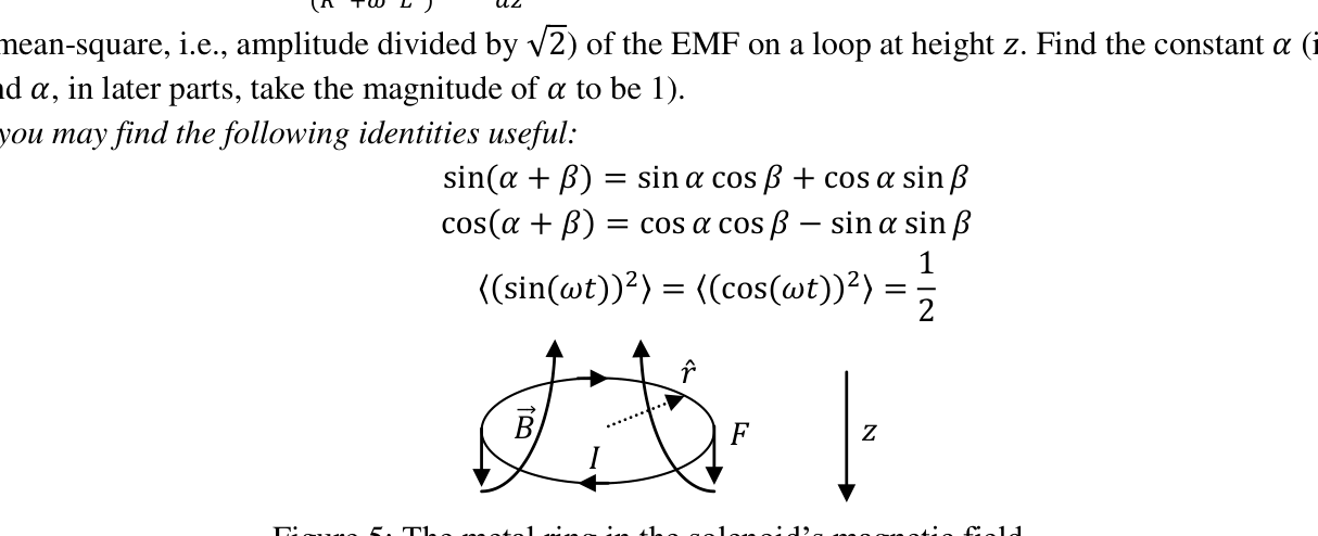
where $I$ is the current in the loop, and $B_r$ is the radial component (in the direction of the loop’s radius) of the external magnetic field in the loop’s vicinity. The positive direction of the force $F$ is downwards — in the $z$ direction. The positive direction of the current $I$ is shown in Figure 5.

a. (0.2 pts.) Consider an oscillating external magnetic flux ${\Phi }_{\mathrm{B}}(t)=\sqrt{2}{\Phi }_{\mathrm{B}}^{\mathrm{rms}}\sin (\omega t)$ through the ring. Find $ϵ(t)$ — the EMF induced by the given flux only, and $I(t)$ — the current induced in the ring, as functions of ${\Phi }_{\mathrm{B}}^{\mathrm{rms}}$, $L$, $R$, $\omega$ and $t$.

Hint: The EMF amplitude ${ϵ}_0$ and the current amplitude $I_0$ on an AC circuit element with both resistance and inductance are related by ${ϵ}_0=I_0\sqrt{{\omega }^2{L}^2+R^2}$, and the current is delayed by a phase $\delta ={\tan }^{-1}\frac{\omega L}{R}$ with respect to the EMF.

b. (0.6 pts.) Find $B_r$ in terms of $r$ and $\frac{d}{dz}{\Phi }_{\mathrm{B}}$, where $z$ is the coordinate along the axis perpendicular to the ring’s plane.

c. (0.5 pts.) Show that $⟨F⟩=\alpha \frac{L}{(R^2+{\omega }^2{L}^2)}\cdot \frac{d({ϵ}_{rms}{)}^2}{dz}$, where $⟨F⟩$ is the time averaged value of $F$, ${ϵ}^{rms}(z)$ is the RMS (root-mean-square, i.e., amplitude divided by $\sqrt{2}$) of the EMF on a loop at height $z$. Find the constant $\alpha$ (if you do not find $\alpha$, in later parts, take the magnitude of $\alpha$ to be 1).

Hint: you may find the following identities useful: $\sin (\alpha +\beta )=\sin \alpha \cos \beta +\cos \alpha \sin \beta$ $\cos (\alpha +\beta )=\cos \alpha \cos \beta -\sin \alpha \sin \beta$ $⟨(\sin (\omega t){)}^2⟩=⟨(\cos (\omega t){)}^2⟩=\frac{1}{2}$

Figure 5 — The metal ring in the solenoid's magnetic field

Measurements (5.1 points)

In all of the following measurements and analysis, take into account that results with higher precision will receive higher grades. In all of your measurements and results, specify error estimations.

Resistance measurements (2.6 points)

In this part, you should use the 0.7 V terminals of the AC power supply. Using the supplied wires to short-circuit the two 0.7 V terminals should result in a current of $5\text{A}-15\text{A}$, depending on the contacts. Note that the three shorter wires achieve a better contact with the ammeter than the two longer ones. CAUTION: Don’t use the 24 V terminals, to avoid overheating the components.

d. (1.3 pts.) Find the resistance $R_{thin}$ of the thin ring. Draw your circuit on the answer form.

Hint: the resistance of each of the rings is much smaller than $0.1\Omega$. For the thin ring, you can neglect the inductive impedance with respect to the resistance.

e. (1.3 pts.) Find the resistance $R$ of the closed ring. Make additional measurements as necessary.

Measurements of the induced EMF (1.5 points)

f. (1.5 pts.) Connect the solenoid to the 24 V terminals of the power supply. Place the broad open ring so that its axis coincides with the axis of the solenoid. Measure the induced EMF ${ϵ}_{rms}$ on the ring at different heights $z$, i.e., at different distances from the solenoid. Record your measurements in the provided table on the answer form. Plot a graph of ${ϵ}_{rms}$ as a function of $z$ (with a trend line).

Measurements of the force (1 point)

g. (1 pt.) Place the broad closed ring so that its axis coincides with the axis of the solenoid. Measure the time-averaged magnetic force $⟨F⟩$ on the ring at different heights $z$, i.e. at different distances from the solenoid. Record your measurements in the provided table on the answer form.

Analysis (3.6 points)

h. (1.4 pts.) Find the absolute value of the derivative $\left|\frac{d{ϵ}_{rms}^2}{dz}\right|$ of ${ϵ}_{rms}^2$ with respect to $z$, for values of $z$ where you measured the force in part (g). Record your values in the provided table on the answer form. Error estimations are not required in this part.

i. (2.2 pts.) Analyze your results using a linear graph to find $L$ — the inductance of the closed ring. You may use the fact that $R=R_{thin}$.

Note: Despite the noticeable thickness of the closed ring, the formula you derived in part (c) still applies with a high accuracy. Use it as an operational definition for the inductance of a broad ring.

Hint: When the ring is too close to the iron, the measurements will be distorted. Try to avoid this complication in your analysis.

Fonte: Testo (PDF) — p.1 Topic: Electromagnetic Induction, Circuits Metodi: Faraday’s Law of Induction, Experimental Data Analysis, Graph Linearization, Error Propagation Competenze: Experimental Data Analysis, Measurement & Instrumentation, Graph Linearization, Error Propagation Objects: Solenoid, Coil

Questione sperimentale 1: Levitamento dei conduttori in un campo magnetico oscillante

In un campo magnetico oscillante di sufficiente forza, la levitazione di un conduttore metallico diventa possibile. La levitazione si verifica a causa di una forza magnetica media non zero esercitata sulle correnti nel conduttore. Le correnti sono indotte dal campo alternativo stesso. La forza di Lorentz non si riduce a zero a causa di un cambiamento di fase tra le oscillazioni di corrente e le oscillazioni del campo magnetico. Questo spostamento di fase è il risultato dell’autoinduzione dei circuiti correnti all’interno del conduttore.

In questo esperimento, studiamo questo fenomeno e deducono l’auto-induzione di un anello di alluminio misurando la forza verticale applicata a esso da un solenoide con una corrente oscillante. Per facilitare la misurazione, la forza media sull’anello sarà diretta verso il basso, quindi non verrà osservata la levitazione.

La carta è costituita da:

1. Un alimentatore a corrente alternata che opera a 50 Hz. La fonte di alimentazione ha due paia di terminali. Le due prese più piccole (1a) forniscono una tensione di circa 24 V; utilizzano queste solo per il flusso di corrente attraverso il solenoide. Le due prese più grandi (1b) forniscono una tensione di circa 0,7 V. L’alimentazione viene attivata solo quando si premono il pulsante verde (1c) questo è per evitare il surriscaldamento del sistema lasciando accidentalmente acceso il corrente, come spiegato in seguito. La lampada rossa indica quando l’alimentazione è accesa.

2. Un solenoide cilindricamente simmetrico riempito di bastone di ferro. Il solenoide è collegato ai terminali 24 V dell’alimentazione. Il solenoide può essere sollevato e abbassato utilizzando una lunga vite. Il passo verticale della vite è $h=1.41\text{mm}$.

3.–5. Tre anelli metallici realizzati esattamente dallo stesso materiale (una lega di alluminio). Un anello è chiuso. Il secondo anello è identico al primo, tranne che un breve segmento che è stato rimosso, rendendo l’anello aperto. Anche il terzo anello è aperto, ed è molto più sottile dei primi due.

6.–7. Due multimetri. Saranno utilizzati come voltometro e ammetro. La sensibilità del voltmeter a corrente alternata è di 0,1 mV. L’ampilometro può misurare correnti fino a 20 A (anche in modalità CA). **Nota: ** in modalità AC, i multimetri mostrano il RMS (root-median-square) della quantità misurata, ovvero: l’ampiezza divisa per $\sqrt{2}$. Per le istruzioni dettagliate, vedere le figure 3 e 4.

8. Una scala digitale alimentata da batterie con sensibilità di 0,01 g. Quando la scala sperimenta una forza che oscilla rapidamente, mostra la forza media temporale. Nota: la scala dispone di un’opzione “tare”, che calibra la lettura sotto un determinato peso a zero. V. figura 2.

9. Un blocco di polistirolo $8\text{cm}\times 7\text{cm}\times 7\text{cm}$ che può essere utilizzato come supporto per gli anelli.

10. Cavi elettrici con diversi connettori.

11. Un governante.

12. Carta grafica millimetrica.

13. Una lampada da scrivania che può essere accesa o spenta per la vostra comodità.

**Certazione: ** quando l’anello chiuso è esposto al campo magnetico del solenoide, una grande corrente fluisce attraverso di esso, riscaldandolo. Di conseguenza, le proprietà elettriche dell’anello possono cambiare leggermente. Per evitare questo, non eseguire una corrente attraverso il solenoide per lunghi periodi di tempo.

Il campo gravitazionale terrestre a Tel Aviv è $g=9.80\pm 0.01\text{N/kg}$.

[figura] Figura 1 Sommario dell’attrezzatura (1) alimentazione a 50 Hz; (1a) terminali 24 V; (1b) terminali 0,7 V; (1c) pulsante di alimentazione. (2) Solenoide su una vite verticale. (3) Anello chiuso largo. (4) Anello largo e aperto. (5) Anello aperto sottile. (6) Voltmeter. (7) Ammetro. (8) Scala. (9) Blocco di polistirolo. (10) Fibri.

[fig.] Figura 2 La scala digitale (1) pulsante accensione/spegnazione. (2) Il pulsante “Tare” imposta il peso corrente come 0.

[figura] Figura 3 Il voltometro (1) pulsante accensione/spegnazione. (2) Il quadrante è impostato a 200 mV di corrente corrente. (3) Connettere i fili ai terminali “COM” e “V/Ω”.

[figura] Figura 4 L’ampilometro (1) pulsante accensione/spegnazione. (2) Il quadrante è impostato a 20 mA / 20 A AC. (3) Connettere i fili ai terminali “COM” e “A”.

Teoria (1.3 punti)

Considerate un anello conduttore di raggio $r$ inserito nel campo magnetico del solenoide. Gli assi di simmetria del solenoide e dell’anello coincidono. Indicare l’inductanza dell’anello di $L$, la sua resistenza di $R$ e la frequenza angolare della corrente del solenoide di $\omega$. Definire $z$ come coordinata lungo l’asse di simmetria comune del solenoide e dell’anello.

Solo in questa parte, si può trascurare il piccolo effetto del campo magnetico dell’anello sul solenoide e sul ferro. Inoltre, trascurate lo spessore dell’anello.

In questa parte, useremo la legge di Faraday, e la versione magnetica della legge di Gauss:

• **Legge di Faraday: ** La forza elettromotrice indotta su un circuito generato da un flusso magnetico mutevole è $ϵ=-d{\Phi }_{\mathrm{B}}/dt$.
• **La legge di Gauss: ** il flusso magnetico totale attraverso una superficie chiusa è zero.

Un circuito corrente posizionato in un campo magnetico cilindricamente simmetrico $\vec{B}$ sperimenta una forza totale

$F(t)=-2\pi rI(t)B_r(t)$

in cui $I$ è la corrente nel ciclo e $B_r$ è la componente radial (in direzione del raggio del ciclo) del campo magnetico esterno nelle vicinanze del ciclo. La direzione positiva della forza $F$ è verso il basso nella direzione $z$. La direzione positiva della corrente $I$ è mostrata alla figura 5.

**a. (0,2 pts) ** Considera un flusso magnetico esterno oscillante ${\Phi }_{\mathrm{B}}(t)=\sqrt{2}{\Phi }_{\mathrm{B}}^{\mathrm{rms}}\sin (\omega t)$ attraverso l’anello. Trova $ϵ(t)$ la FEM indotta solo dal flusso dato e $I(t)$ la corrente indotta nell’anello, come funzioni di ${\Phi }_{\mathrm{B}}^{\mathrm{rms}}$, $L$, $R$, $\omega$ e $t$.

Signore: L’ampiezza EMF ${ϵ}_0$ e l’ampiezza corrente $I_0$ su un elemento di circuito AC con resistenza e induttanza sono correlati da ${ϵ}_0=I_0\sqrt{{\omega }^2{L}^2+R^2}$, e la corrente è ritardata da una fase $\delta ={\tan }^{-1}\frac{\omega L}{R}$ rispetto all’EMF.

**b. (0,6 punti) ** Trova $B_r$ in termini di $r$ e $\frac{d}{dz}{\Phi }_{\mathrm{B}}$, dove $z$ è la coordinata lungo l’asse perpendicolare al piano dell’anello.

**c. (0,5 punti) ** Indicare che $⟨F⟩=\alpha \frac{L}{(R^2+{\omega }^2{L}^2)}\cdot \frac{d({ϵ}_{rms}{)}^2}{dz}$, dove $⟨F⟩$ è il valore medio temporale di $F$, ${ϵ}^{rms}(z)$ è il RMS (raggine-media-quadrato, cioè amplitudine divisa da $\sqrt{2}$) del FEM su un ciclo ad altezza $z$. Trova la costante $\alpha$ (se non trovi $\alpha$, nelle parti successive, prendi la magnitudine di $\alpha$ per essere 1).

Signore: potresti trovare utili le seguenti identità: $\sin (\alpha +\beta )=\sin \alpha \cos \beta +\cos \alpha \sin \beta$ $\cos (\alpha +\beta )=\cos \alpha \cos \beta -\sin \alpha \sin \beta$ $⟨(\sin (\omega t){)}^2⟩=⟨(\cos (\omega t){)}^2⟩=\frac{1}{2}$

[fig. 5] Figura 5 L’anello metallico nel campo magnetico del solenoide

Misure (5,1 punti)

In tutte le seguenti misurazioni e analisi, si deve tenere conto che i risultati con maggiore precisione riceveranno voti più elevati. In tutte le misure e i risultati, specificare le stime di errore.

Misure della resistenza (2,6 punti)

In questa parte, è necessario utilizzare i terminali di 0,7 V dell’alimentazione a corrente alternata. L’utilizzo dei fili forniti per il cortocircuito dei due terminali di 0,7 V dovrebbe comportare una corrente di $5\text{A}-15\text{A}$, a seconda dei contatti. Si noti che i tre fili più brevi raggiungono un migliore contatto con l’ampimetro rispetto ai due fili più lunghi. **Caution: ** Non utilizzare i terminali 24 V, per evitare il surriscaldamento dei componenti.

**d. 1, 3 punti) ** Trova la resistenza $R_{thin}$ dell’ anello sottile. Disegna il circuito sul modulo di risposta.

*Signore: * la resistenza di ciascuno degli anelli è molto inferiore a $0.1\Omega$. Per l’anello sottile, si può trascurare l’impedenza induttiva rispetto alla resistenza.

**e. 1, 3 punti) ** Trova la resistenza $R$ dell’ anello chiuso. Fare ulteriori misure se necessario.

Misure del FEM indotto (1,5 punti)

f. 1, 5 pts.) Collegare il solenoide ai terminali 24 V dell’alimentazione. Si colloca l’anello aperto ampio in modo che il suo asse coincida con l’asse del solenoide. Misurare la EMF ${ϵ}_{rms}$ indotta sull’anello ad altezze diverse $z$, cioè a distanze diverse dal solenoide. Registrare le misure nella tabella fornita sul modulo di risposta. Tracciare un grafico di ${ϵ}_{rms}$ come funzione di $z$ (con una linea di tendenza).

Misure della forza (1 punto)

g. (1 pt.) Metti l’anello chiuso largo in modo che il suo asse coincida con l’asse del solenoide. Misurare la forza magnetica media temporale $⟨F⟩$ sull’anello a diverse altezze $z$, ovvero a distanze diverse dal solenoide. Registrare le misure nella tabella fornita sul modulo di risposta.

analisi (3,6 punti)

**h. 1, 4 punti.) ** Trova il valore assoluto della derivata $\left|\frac{d{ϵ}_{rms}^2}{dz}\right|$ di ${ϵ}_{rms}^2$ rispetto a $z$, per i valori di $z$ in cui hai misurato la forza in parte (g). Registrare i valori nella tabella fornita sul modulo di risposta. In questa parte non sono richieste stime di errore.

**i. (2,2 punti) ** Analizzare i risultati utilizzando un grafico lineare per trovare $L$ l’induttanza dell’anello chiuso. È possibile utilizzare il fatto che $R=R_{thin}$.

Nota: Nonostante l’espansione notevole dell’anello chiuso, la formula derivata dalla parte (c) si applica ancora con elevata precisione. Utilizzare come definizione operativa per l’induzione di un anello ampio.

*Signore: * Quando l’anello è troppo vicino al ferro, le misure saranno distorte. Cerca di evitare questa complicazione nella tua analisi.

Fonte: Testo (PDF) — p.1 Topic: Electromagnetic Induction, Circuits Metodi: Faraday’s Law of Induction, Experimental Data Analysis, Graph Linearization, Error Propagation Competenze: Experimental Data Analysis, Measurement & Instrumentation, Graph Linearization, Error Propagation Objects: Solenoid, Coil

Experimental Question 2: An Optical “Black Box”

TV and computer screens have advanced significantly in recent years. Today, most displays consist of a color LCD filter matrix and a uniform white backlight source. In this experiment, we will study a sample of plastic material which was considered for use as an ingredient in the backlight illumination of LCD screens.

Equipment

On your desk, you have the following items (see Figure 1):

1. The sample — a piece of plastic material fixed in a slide frame. The sample is sensitive — do not touch it. To adjust the sample’s position, use its holder and stand.

2. A holder and stand for the slide frame. The stand includes a handle which can be used for fine rotations of the sample. Do not remove the slide frame from its holder.

3. A white LED flashlight. The flashlight can be turned on and off using a button at its rear end. Do not confuse it with the laser (see Figure 2).

4. A red laser pointer. The laser is marked with a warning label. Do not confuse it with the white flashlight (see Figure 2). The laser may be turned on and off by moving its black cap back and forth. Don’t try to remove the cap — it may be dangerous, and you may break the laser. The laser’s battery will weaken after about an hour — do not keep it turned on longer than necessary. The laser’s wavelength is $\lambda =652\text{nm}\pm 2\text{nm}$.

5. A single stand to be used for the two light sources. At the start of the experiment, the flashlight is fixed to the stand, while the laser lies on the desk.

6. A white screen on wooden legs, covered with millimeter graph paper. There is a hole near the middle of the screen. You are allowed to make markings on the screen.

7. A wooden stake that can be moved back and forth on a wooden bench. You are allowed to make markings on the bench.

8. A tape measure.

9. A ruler.

10. Millimeter graph paper.

11. A desktop lamp which can be turned on or off for your convenience.

LASER SAFETY:

1. Do not stare into the laser beam!
2. Beware of reflections from metallic surfaces.
3. Do not point the laser at others.
4. Do not try to repair or disassemble the laser.

Call a supervisor if you require assistance.

Figure 1 — Summary of the equipment

(1) The plastic sample. (2) Sample holder and stand. (3) White LED flashlight. (4) Red laser. (5) Stand for light source. (6) Screen covered with millimeter graph paper. (7) Wooden stake on bench. (8) Tape measure.

Figure 2 — Close-up of the two light sources

(3) White flashlight. (4) Red laser.

Part I — Theory (0.4 points)

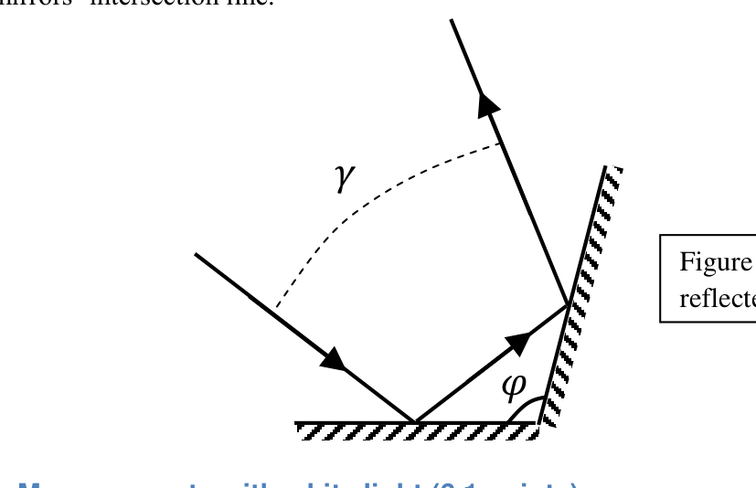
a. (0.4 pts.) A light ray is reflected from two mirrors which meet at an angle $\phi$ (Figure 3). Find the angle $\gamma$ between the incoming and outgoing rays. Assume that all light rays lie in the plane perpendicular to the mirrors’ intersection line.

Figure 3 — A light ray reflected from two mirrors

Part II — Measurements with white light (6.1 points)

Using the white flashlight as your light source, you may observe both the transmission and the reflection properties of the sample. Figure 4 illustrates the suggested setups for both types of observation. Note: you may observe different results when illuminating the two sides of the sample.

CAUTION: For viewing transmitted light, you will have to look directly into the flashlight beam through the sample. Don’t do this with the laser! Also, avoid looking directly into the flashlight itself for long periods of time.

Figure 4 — Suggested observation setups for white light

Transmission: Eye — Sample — White flashlight. Reflection: White flashlight — Sample — Screen.

b. (0.5 pts.) Figure 5 illustrates schematically four possibilities for the sample’s microscopic structure. $n$ stands for the refractive index of the plastic. Choose the structure that best fits your observations. Note: the 5 periods shown in the figure are for illustration only. In reality, $d$ is small, and the sample contains many periods.

Figure 5 — Different possibilities for the sample's structure

(A) Symmetric triangular grooves (period $d$, angle $\phi$). (B) Symmetric grooves with flat tops (groove width $d/2$, period $d$, angle $\phi$). (C) Asymmetric sawtooth with flat tops (width $d/2$, period $d$, angle $\phi$). (D) Asymmetric sawtooth (blazed) profile (period $d$, angle $\phi$).

c. (0.8 pts.) Find the angle $\phi$ for the sample and estimate its error.

d. (0.5 pts.) When a perpendicular white light beam is incident on the sample from one of its sides, the following faint pattern can be observed in the transmitted light, slightly to the right from the source (Figure 6). “R”, “G” and “B” stand for red, green and blue respectively. Note: this pattern may be difficult to observe, and measurements on it are not required.

Figure 6 — Faint pattern near the light source

Repeated “BGR” colored groups to the right of the source.

Further to the right you may observe a much brighter pattern (Figure 7):

Figure 7 — Bright pattern farther to the right from the light source

A single bright “R G B” sequence.

Choose the correct option:

• A. All the colored patterns result from interference.
• B. All the colored patterns result from the dependence of $n$ on the wavelength.
• C. The patterns depicted in Figure 6 result from interference, while the pattern depicted in Figure 7 results from dependence of $n$ on the wavelength.
• D. The patterns depicted in Figure 6 result from the dependence of $n$ on the wavelength, while the pattern depicted in Figure 7 results from interference.

e. (1.4 pts.) With the white light set up as in part (d), measure the deflection angle ${\delta }_0$ of violet light (at the far blue end of the spectrum) for the dominant peak depicted in Figure 7. The deflection angle is defined in Figure 8. Record all intermediate measurements. Provide error estimates.

Figure 8 — The deflection angle ${\delta }_0$

Light incident perpendicularly on the sample is transmitted and deflected by an angle ${\delta }_0$ from the original direction.

f. (1.4 pts.) Illumination of the sample at different angles of incidence results in different deflection angles for the dominant transmitted peaks. Measure the minimal deflection angle ${\delta }_{min}$ of the dominant peak for transmitted violet light (there is only one such minimal angle). Record all intermediate measurements. Provide error estimates.

g. (0.8 pts.) Using the angle $\phi$ from part (c), express the refraction index $n$ of the sample in terms of either ${\delta }_0$ or ${\delta }_{min}$. You may use the reversibility of light propagation and the fact that there is only one minimal angle ${\delta }_{min}$.

h. (0.7 pts.) Find the refraction index $n_v$ of the sample for violet light and its error estimate.

Part III — Laser measurements (3.5 points)

Remove the flashlight from the light-source stand, and replace it with the laser. You can use the white screen to view both transmission and reflection patterns, as illustrated in Figure 9. The laser has a limited battery life — do not keep it turned on longer than necessary. When aligning the components, it may help to rotate the laser around its axis.

WARNING: Do not look directly into the laser beam or its reflections! Do not look at the laser light through the sample — use the provided screen.

Figure 9 — Suggested observation setups for laser light

Transmission: Laser — Sample — Screen. Reflection: Laser/Sample — Screen.

Observe the alternating pattern of bright and dim fringes on the screen as you slightly rotate the sample. The dimming of some of the fringes is due to destructive interference between different regions of each “tooth” on the sample.

i. (1 pt.) Use one of the setups in Figure 9, with the sample illuminated perpendicularly by the laser beam. Record the deflection angles $\theta$ of the observed fringes as a function of the fringe number $m$. Define the center of the pattern as $m=0$. Use the provided table on the answer form. Record all intermediate measurements. Provide error estimations.

j. (1.5 pts.) Using a linear graph, find the spacing $d$ between two adjacent “teeth” of the sample. Error bars on the graph are not required. Provide error estimation for $d$.

k. (1 pt.) Using the formula you derived in part (g), find the refraction index $n_r$ of the sample for the laser’s red wavelength. Record any additional measurements. Provide error estimates. WARNING: Do not look through the sample! Use the provided screen.

Fonte: Testo (PDF) — p.1 Topic: Wave Optics, Geometric Optics Metodi: Interference & Diffraction Analysis, Snell’s Law, Experimental Data Analysis, Graph Linearization Competenze: Experimental Data Analysis, Measurement & Instrumentation, Graph Linearization, Error Propagation Objects: Diffraction Grating, Mirror, Screen

Domanda sperimentale 2: “Scatola nera” ottica

Negli ultimi anni i televisori e gli schermi dei computer hanno fatto notevoli progressi. Oggi la maggior parte dei display sono costituiti da una matrice di filtro LCD a colori e da una fonte uniforme di retroilluminazione bianca. In questo esperimento, studieremo un campione di materiale plastico che è stato considerato per l’uso come ingrediente nell’illuminazione a retro dei schermi LCD.

Equipaggiamento

La carta è costituita da:

1. Il campione è un pezzo di materiale plastico fissato in una cornice. Il campione è sensibile non toccarlo. Per regolare la posizione del campione, utilizzare il suo tenore e il suo supporto.

2. Un supporto e un supporto per la cornice. Il supporto comprende una maniglia che può essere utilizzata per le rotative sottili del campione. Non togliere il telaio della diapositiva dal suo contenitore.

3. Una lampada da fuoco LED bianca. La torcia può essere accesa o spenta con un pulsante nella sua parte posteriore. Non confondere con il laser (vedere figura 2).

4. Un puntatore laser rosso. Il laser è contrassegnato con un’etichetta di avvertimento. Non confondere con la lampada da fuoco bianca (vedere figura 2). Il laser può essere acceso e spento spostando il suo cappotto nero avanti e indietro. Non cercare di rimuovere il cappuccio. Può essere pericoloso e si può rompere il laser. La batteria del laser si indebolirà dopo circa un’ora. La lunghezza d’onda del laser è $\lambda =652\text{nm}\pm 2\text{nm}$.

5. Un unico supporto da utilizzare per le due fonti di luce. All’inizio dell’esperimento, la lanterna è fissata al banco, mentre il laser si trova sulla scrivania.

6. Uno schermo bianco su gambe di legno, ricoperto di carta grafica millimetrica. C’è un buco vicino al centro dello schermo. È permesso fare segni sullo schermo.

7. Un palo di legno che si può spostare avanti e indietro su una panchina di legno. Ti e’ permesso fare i segni sulla panchina.

8. Un nastro di misura.

9. Un governante.

10. Carta grafica millimetrica.

11. Una lampada da scrivania che può essere accesa o spenta per la vostra comodità.

**SAFETY FOR LASER: **

1. Non fissare il raggio laser!
2. Attenzione ai riflessi da superfici metalliche.
3. Non puntare il laser sugli altri.
4. Non cercare di riparare o smontare il laser.

Chiamate un supervisore se avete bisogno di assistenza.

[figura] Figura 1 Sommario dell’attrezzatura (1) Il campione di plastica. (2) Tinta e supporto del campione. (3) Lanterna a LED bianca. (4) Laser rosso. (5) Fate riferimento alla fonte di luce. (6) schermo ricoperto di carta grafica millimetrica. (7) Pilo di legno su una panchina. (8) misura del nastro.

[figura] Figura 2 Rappresentazione rapida delle due fonti luminose (3) Lanterna bianca. (4) Laser rosso.

Parte I Teoria (0,4 punti)

**a. (0,4 pts.) ** Un raggio luminoso è riflesso da due specchi che si incontrano ad un angolo $\phi$ (Figura 3). Trova l’angolo $\gamma$ tra i raggi entranti e usciti. Supponiamo che tutti i raggi luminosi si trovino nel piano perpendicolare alla linea di intersezione degli specchi.

[figura] Figura 3 Un raggio di luce riflesso da due specchi

Parte II Misure con luce bianca (6,1 punti)

Usando la lampada da fuoco bianca come fonte di luce, si possono osservare sia la trasmissione che le proprietà di riflessione del campione. La figura 4 illustra le impostazioni proposte per entrambi i tipi di osservazione. Nota:* si possono osservare risultati diversi quando si illuminano i due lati del campione.

**Caution: ** Per visualizzare la luce trasmessa, dovrai guardare direttamente nel raggio della lampada da fuoco attraverso il campione. Non farlo con il laser! Inoltre, non guardare direttamente la lampada da fuoco per lunghi periodi di tempo.

[figura] Figura 4 Configurazioni di osservazione suggerite per la luce bianca Trasmissione: occhio campione lampada da fuoco bianca. Riflessione: lampada bianca campione schermo.

b. (0,5 pts.) La figura 5 illustra schematicamente quattro possibilità per la struttura microscopica del campione. $n$ indica l’indice di rifrazione della plastica. Scegli la struttura che meglio si adatta alle tue osservazioni. *Nota: * i 5 periodi indicati nella figura sono solo per esempio. In realtà, $d$ è piccolo e il campione contiene molti periodi.

[figura] Figura 5 Diverse possibilità per la struttura del campione (A) Stiglie triangolari simmetriche (periodo $d$, angolo $\phi$). (B) Sceneggiature simmetriche con punte piatte (larghezza del sceneggiamento $d/2$, periodo $d$, angolo $\phi$). (C) Denti di seggia asimmetrici con coppie piatte (larghezza $d/2$, periodo $d$, angolo $\phi$). D) Profil di dente di seggia (a gonfiore) asimmetrico (periodo $d$, angolo $\phi$).

**c. (0,8 punti di punto) ** Trova l’angolo $\phi$ del campione e stima il suo errore.

d. (0,5 pts.) Quando un fascio di luce bianca perpendicolare incide sul campione da uno dei suoi lati, nel luminoso trasmesso si può osservare il seguente modello debole, leggermente a destra dalla sorgente (Figura 6). “R”, “G” e “B” sono rispettivamente rosso, verde e blu. Nota: questo modello può essere difficile da osservare e non sono necessarie misure su di esso.

[figura] Figura 6 Modello debole vicino alla fonte luminosa Gruppi colorati “BGR” ripetuti a destra della fonte.

Più avanti a destra si può osservare un modello molto più luminoso (Figura 7):

[figura] Figura 7 Disegno luminoso più a destra dalla fonte luminosa Una singola sequenza brillante “R G B”.

Scegliere l’ opzione corretta:

• A. Tutti i modelli colorati sono il risultato di interferenze.
• B. Tutti i modelli colorati derivano dalla dipendenza di $n$ dalla lunghezza d’onda.
• C. I modelli raffigurati nella figura 6 sono risultati di interferenze, mentre il modello raffigurato nella figura 7 è risultato dalla dipendenza di $n$ dalla lunghezza d’onda.
• D. I modelli raffigurati nella figura 6 risultano dalla dipendenza di $n$ dalla lunghezza d’onda, mentre il modello raffigurato nella figura 7 deriva da interferenze.

**e. (1,4 punti) ** Con la luce bianca impostata come nella parte (d), misurare l’angolo di deflessione ${\delta }_0$ della luce viola (all’estremo fine blu dello spettro) per il picco dominante raffigurato nella figura 7. L’angolo di deflezione è definito nella figura 8. Registrare tutte le misure intermedi. Fornire stime di errore.

[figura] Figura 8 L’angolo di deflessione ${\delta }_0$ L’incidente luminoso perpendicolare sul campione viene trasmesso e deviato da un angolo ${\delta }_0$ dalla direzione originale.

**f. L’illuminazione del campione a diverse angolazioni di incidenza comporta angoli di deviazione diversi per i picchi trasmessi dominanti. Misurare l’angolo di deviazione minimo ${\delta }_{min}$ del picco dominante per la luce viola trasmessa (esiste un solo angolo minimo). Registrare tutte le misure intermedi. Fornire stime di errore.

**g. (0,8 pts.) ** Utilizzando l’angolo $\phi$ della parte (c), esprimere l’indice di rifrazione $n$ del campione in termini di ${\delta }_0$ o ${\delta }_{min}$. È possibile utilizzare la reversibilità della propagazione della luce e il fatto che esiste un solo angolo minimo ${\delta }_{min}$.

**h. (0,7 pts.) ** Trova l’indice di rifrazione $n_v$ del campione per la luce viola e la sua stima di errore.

Parte III Misurazioni laser (3,5 punti)

Rimuovi la lanterna dal supporto della fonte luminosa e sostituiscilo con il laser. È possibile utilizzare lo schermo bianco per visualizzare sia i modelli di trasmissione che di riflessione, come illustrato nella Figura 9. Il laser ha una durata limitata della batteria non tenerlo acceso più a lungo del necessario. Quando si allineano i componenti, può aiutare a ruotare il laser attorno al suo asse.

** AVVERTORE: ** Non guardare direttamente il fascio laser o i suoi riflessi! Non guardare la luce laser attraverso il campione utilizzare lo schermo fornito.

[figura] Figura 9 Impostazioni di osservazione suggerite per la luce laser Trasmissione: Laser campione schermo. Riflessione: Laser/Sampolo schermo.

Osservate il modello alternativo di margini luminosi e deboli sullo schermo mentre ruotate leggermente il campione. L’oscurazione di alcuni margini è dovuta ad interferenze distruttive tra le diverse regioni di ciascun “dente” del campione.

i. (1 pt.) Utilizzare una delle configurazioni riportate nella figura 9, con il campione illuminato perpendicolare dal fascio laser. Registrare gli angoli di deviazione $\theta$ dei margini osservati come funzione del numero di margine $m$. Definire il centro del modello come $m=0$. Utilizzare la tabella fornita sul modulo di risposta. Registrare tutte le misure intermedi. Fornire stime di errore.

**j. (1,5 punti) ** Usando un grafico lineare, trovare l’intervallo $d$ tra due “denti” adiacenti del campione. Le barre di errore sul grafico non sono necessarie. Fornire la stima di errore per $d$.

k. (1 pt.) Usando la formula derivata dalla parte (g), trovare l’indice di rifrazione $n_r$ del campione per la lunghezza d’onda rossa del laser. Registrare eventuali misure aggiuntive. Fornire stime di errore. ** AVVERTORE: ** Non guardare attraverso il campione! Utilizzare lo schermo fornito.

Fonte: Testo (PDF) — p.1 Topic: Wave Optics, Geometric Optics Metodi: Interference & Diffraction Analysis, Snell’s Law, Experimental Data Analysis, Graph Linearization Competenze: Experimental Data Analysis, Measurement & Instrumentation, Graph Linearization, Error Propagation Objects: Diffraction Grating, Mirror, Screen