APhO 2012 — Sperimentale

FRICTION

If a cord is passed around a post or a beam and the tensions in the two segments are different, friction between the cord and the beam plays a role in controlling the motion of the cord (Fig.1). It is observed that to hold a body suspended at one end of the cord, the minimum force needed at the other end of the cord is less than the weight of the body due to the presence of frictional forces. With the increase in the number of turns around the beam the decrease in force is spectacular. Sailors are known to use this idea for arresting the motion of ships by winding ropes tied to ships around posts at the docks.

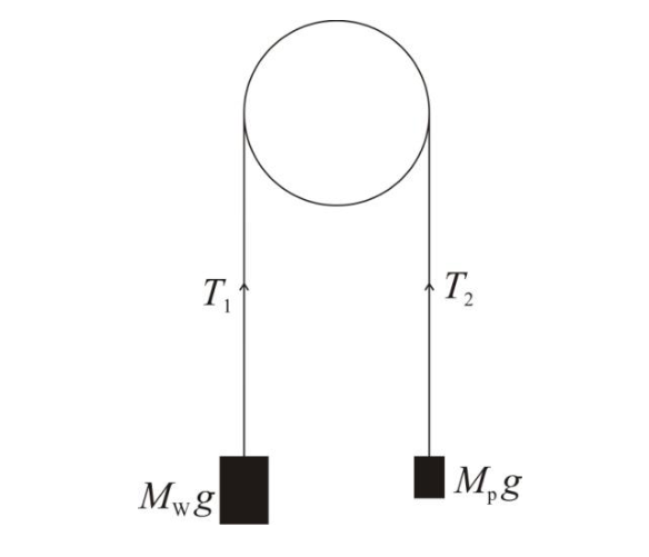
Fig.1

Objective:

To explore the relationship among the three quantities: the load $W(=M_{\mathrm{w}}g)$, the minimum effort $P(=M_{\mathrm{p}}g)$ needed to keep the system in equilibrium and the angle $\theta$, subtended by the segment of the cord in contact with one or more beams, by systematically varying these quantities and to express it in the form of an equation.

Apparatus:

Sr. No.	Item	Quantity
1	An apparatus consisting of four pieces of steel pipe on four sides of an identical vertical piece at the centre, all fixed on a wooden platform	1
2	An acrylic sheet (with lines 1.5 mm apart) mounted in front of one of the horizontal pipes	1
3	A plastic pan (including supporting rods) with its mass ($M_{\text{pan}}$) written on its side	1
4	A magnifying glass with torch	1
5	White cord with blue markings (Dial cord)	2 pieces
6	Pink cord	1 piece
7	A weight box containing following weights
	500.0 g	1
	200.0 g	2
	100.0 g	1
	50.0 g	1
	20.0 g	2
	10.0 g	1
	5.0 g	1
	2.0 g	2
	1.0 g	1
8	A body of unknown mass, $M_x$	1
9	A hanger of slotted weights with hook (each weight 100.0 g and total weight 800.0 g)	1
10	A piece of cleaning cloth	1

The blue switch can be moved to switch the torch ON/OFF. The acrylic plate with lines ruled on it is provided to detect the motion of the cord. The lines on the acrylic plate can be taken as reference against which the motion of the cord can be observed.

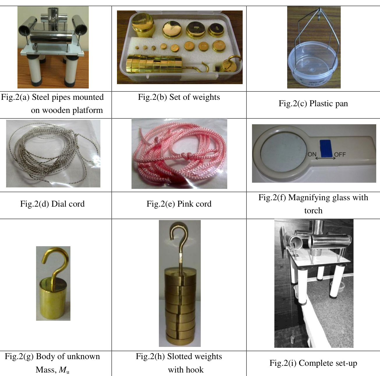
Fig.2(a) Steel pipes mounted on wooden platform — Fig.2(b) Set of weights — Fig.2(c) Plastic pan — Fig.2(d) Dial cord — Fig.2(e) Pink cord — Fig.2(f) Magnifying glass with torch — Fig.2(g) Body of unknown Mass, $M_x$ — Fig.2(h) Slotted weights with hook — Fig.2(i) Complete set-up

Experimental Procedure:

Caution: Do not touch the surface of the pipes with which the cord would be in contact. Any greasy material can change the frictional properties of the surface (surface of the pipes as well as the cord). A cleaning cloth is provided if required.

Part 1:

(Note: Use the dial cord in this part.)

Use the hanger with slotted weights as load $M_{\mathrm{w}}$. Attach the load at one end of the given piece of dial cord (whose mass is negligible) and a pan (with known mass) at the other. A weight box with weights is also provided. The angle $\theta$ subtended by the cord can be changed by passing it over/around two or more of the given pipes. (Refer Fig.3).

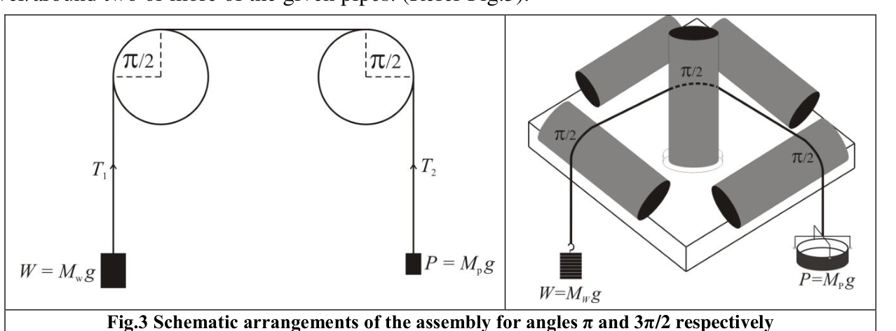
The minimum value of angle $\theta$ is obtained when the cord passes over two parallel rods without making any contact with the central post (Fig.3). By winding the cord around the vertical post and shifting the position of the effort the angle $\theta$ can be changed by steps of $\pi /2$. The load $M_{\mathrm{w}}$ should be suspended from the pipe to which the ruled acrylic plate is mounted.

For increasing the angle $\theta$ the cord is to be turned around the central vertical post. To observe whether the cord suspending the load is slipping over the pipe, the transparent acrylic plate is provided. You can use the magnifying glass with torch to view whether the cord is slipping over the pipe. Ideally one should note the effort $M_{\mathrm{p}}$ when the load $M_{\mathrm{w}}$ is on the verge of moving down (overcoming static friction). But that is not possible. However, it is possible to determine the interval $[M_{p1},M_{p2}]$ within which this value lies. Since this interval is a measure of the uncertainty in the magnitude of $M_{\mathrm{p}}$, it should be made as small as possible.

For $\theta =\pi$, take observations over as wide range as possible with the weights provided. Make estimate of the uncertainties in the observations. Plot the necessary graphs and combine the results from the graphs to get the desired equation. On the basis of the analysis of your data write down the quantitative relation giving value of $P$ in terms of $W$ and $\theta$. The value of $P$ is also dependent on friction between the cord and the pipe. Identify the term in your equation which accounts for friction and equate it to the coefficient of friction $\mu$ for the given system. Estimate the expanded uncertainty in its value.

Part 2:

(Note: Use the pink cord in this part.)

A body of unknown mass $M_x$ and a pink cord is provided. Suspend the unknown mass from one end of the cord and the pan from the other end. Write down the relevant equations to determine $M_x$ and ${\mu }_x$. With $\theta =\pi$, take necessary observations to determine its mass and the coefficient of friction between the pink cord and the pipes using the relationship obtained in the experiment. Estimate the expanded uncertainty in your results.

Note on uncertainty evaluation

1. If it is observed that the magnitude $X$ of a quantity to be measured lies somewhere in an interval $[X_1,X_2]$, and there is equal probability that it can have any value in this interval, then the probability distribution is said to be uniform or rectangular. The standard uncertainty for such distribution is given by $\frac{|X_1-X_2|}{2\sqrt{3}}$.

2. After evaluating the combined standard uncertainty in a measured quantity, the result is stated with an expanded uncertainty. The expanded uncertainty is taken equal to twice the combined standard uncertainty, the confidence level is approximately 95 %. The number giving expanded uncertainty is rounded upwards to retain a single digit (generally) and the number giving the magnitude of the measured quantity is rounded to keep appropriate number of digits such that the last digit has the same decimal place as that of the expanded uncertainty.

Fonte: Testo (PDF) — p.1 Topic: Newtonian Mechanics, Rigid Body Statics Metodi: Free-Body Diagram, Experimental Data Analysis, Graph Linearization, Error Propagation Competenze: Experimental Data Analysis, Measurement & Instrumentation, Error Propagation, Graph Linearization Objects: String, Tube

---

Friczione

Se un cavo viene trasmesso attorno a un palo o a un raggio e le tensioni nei due segmenti sono diverse, l’attrito tra il cavo e il raggio svolge un ruolo nel controllo del movimento del cavo (Fig.1). Si osserva che per tenere un corpo sospeso ad una estremità del cordone, la forza minima necessaria all’altra estremità del cordone è inferiore al peso del corpo a causa della presenza di forze di attrito. Con l’aumento del numero di giri intorno al fascio la diminuzione della forza è spettacolare. I marinai sono noti per usare questa idea per arrestare il movimento delle navi facendo rotolare le corde legate alle navi intorno ai posti dei porti.

Fig.1

**Obiettivo: **

Per esplorare la relazione tra le tre quantità: il carico $W(=M_{\mathrm{w}}g)$, l’impegno minimo $P(=M_{\mathrm{p}}g)$ necessario per mantenere l’equilibrio del sistema e l’angolo $\theta$, sottoscritto dal segmento del cavo in contatto con uno o più travi, variando sistematicamente tali quantità e esprimendolo sotto forma di equazione.

Apparecchiatura:

| Sr. No. # Il numero di articoli # # Quantità di articoli # |---|---|---| Un apparecchio composto da quattro pezzi di tubo d’acciaio su quattro lati di un pezzo verticale identico al centro, tutti fissati su una piattaforma di legno. ∙ 2 ∙ Un foglio di acrilico (con linee a 1,5 mm di distanza) montato davanti a uno dei tubi orizzontali ∙ 1 ∙ ∙ 3 ∙ Una vasca di plastica (compresi le barre di supporto) con la sua massa ($M_{\text{pan}}$) scritta sul lato ∙ 1 ∙ 4 Una lente di ingrandimento con torcia 1 5 Cordon bianco con marcature blu (Cordon di dial) 2 pezzi

6 # Cordon rosa # 1 pezzo

7 Una scatola di pesi contenente i seguenti pesi | | 500.0 g | 1 | | | 200.0 g | 2 | | | 100.0 g | 1 | | | 50.0 g | 1 | | | 20.0 g | 2 | | | 10.0 g | 1 | | | 5.0 g | 1 | | | 2.0 g | 2 | | | 1.0 g | 1 | | 8 | A body of unknown mass, $M_x$ | 1 | ➡️ Un appeso di pesi a slot con gancio (per peso 100,0 g e peso totale 800,0 g) ➡️ 1 ➡️

Un pezzo di stoffa da pulizia

Il pulsante blu può essere spostato per accendere o spegnere la torcia. La piastra acrilica con le linee regolata è fornita per rilevare il movimento del cavo. Le linee della piastra acrilica possono essere prese come riferimento contro le quali si può osservare il movimento del cavo.

Fig.2(a) Steel pipes mounted on wooden platform — Fig.2(b) Set of weights — Fig.2(c) Plastic pan — Fig.2(d) Dial cord — Fig.2(e) Pink cord — Fig.2(f) Magnifying glass with torch — Fig.2(g) Body of unknown Mass, $M_x$ — Fig.2(h) Slotted weights with hook — Fig.2(i) Complete set-up

Procedura sperimentale:

**Cauzione: ** Non toccare la superficie dei tubi con cui il cavo sarebbe in contatto. Qualsiasi materiale grassi può modificare le proprietà di attrito della superficie (superficia dei tubi e del cavo). Se necessario, viene fornito un panno da pulizia.

Parte 1:

(Nota: utilizzare il cavo di scheda in questa parte.)

Utilizzare il pendolo con pesi a fessura $M_{\mathrm{w}}$ come carico. Appiccare il carico ad una estremità del taglio di cavo di scheda (la cui massa è trascurabile) e un pannello (con massa nota) all’altra. È inoltre fornita una scatola con pesi. L’angolo $\theta$ sottoscritto dal cavo può essere modificato passandolo sopra/circondando due o più dei tubi dati. (Rif. 3).

Il valore minimo di angolo $\theta$ è ottenuto quando il cavo passa su due barre parallele senza alcun contatto con il ponte centrale (Fig.3). By winding the cord around the vertical post and shifting the position of the effort the angle $\theta$ can be changed by steps of $\pi /2$. Il carico $M_{\mathrm{w}}$ deve essere sospeso dal tubo a cui è montata la piastra acrilica a rotura.

Per aumentare l’angolo $\theta$ il cavo deve essere girato attorno al polo verticale centrale. Per osservare se il cavo che sospende il carico scivola sopra il tubo, viene fornita una piastra acrilica trasparente. Puoi usare la lente di ingrandimento con torcia per vedere se il cavo si scivola sopra il tubo. Idealmente si deve notare lo sforzo $M_{\mathrm{p}}$ quando il carico $M_{\mathrm{w}}$ è sull’orlo di scendere (superando lo attrito statico). Ma non è possibile. Tuttavia, è possibile determinare l’intervallo $[M_{p1},M_{p2}]$ entro il quale si trova questo valore. Poiché questo intervallo è una misura dell’incertezza nella magnitudine di $M_{\mathrm{p}}$, deve essere ridotto il più possibile.

Per $\theta =\pi$, effettuare osservazioni su un intervallo più ampio possibile con i pesi forniti. Estimare le incertezze delle osservazioni. Tracciare i grafici necessari e combinare i risultati dei grafici per ottenere l’equazione desiderata. Sulla base dell’analisi dei dati, annotare la relazione quantitativa che dà valore di $P$ in termini di $W$ e $\theta$. Il valore di $P$ dipende anche dalla frizione tra il cavo e il tubo. Identificare il termine nella sua equazione che contiene l’attrito e equipararlo al coefficiente di attrito $\mu$ per il sistema dato. Estimare l’incertezza di valore.

Parte 2:

*(Nota: utilizzare il cavo rosa in questa parte.) *

Si fornisce un corpo di massa sconosciuta $M_x$ e un cavo rosa. Suspendere la massa sconosciuta da un’altra parte del cavo e la padella dall’altra. Scrittore delle equazioni pertinenti per determinare $M_x$ e ${\mu }_x$. Con $\theta =\pi$, effettuare le osservazioni necessarie per determinare la sua massa e il coefficiente di attrito tra il cavo rosa e i tubi utilizzando la relazione ottenuta nell’esperimento. Estima l’incertezza crescente dei risultati.

Nota sull’evaluare l’incertezza

1. Se si osserva che la magnitudine $X$ di una quantità da misurare si trova da qualche parte in un intervallo $[X_1,X_2]$, e che vi è la stessa probabilità che possa avere un valore in questo intervallo, allora la distribuzione di probabilità è considerata uniforme o rettangolare. L’incertezza standard per tale distribuzione è data da $\frac{|X_1-X_2|}{2\sqrt{3}}$.

2. Dopo aver valutato l’incertezza standard combinata in una quantità misurata, il risultato viene indicato con un’incertezza ampliata. L’incertezza ampliata è considerata pari al doppio dell’incertezza standard combinata, il livello di fiducia è di circa il 95%. Il numero che dà l’incertezza ampliata viene arrotondato verso l’alto per mantenere una singola cifra (in genere) e il numero che dà la grandezza della quantità misurata viene arrotondato per mantenere un numero appropriato di cifre in modo tale che l’ultima cifra abbia la stessa decimale della incertezza ampliata.

Fonte: Testo (PDF) — p.1 Topic: Newtonian Mechanics, Rigid Body Statics Metodi: Free-Body Diagram, Experimental Data Analysis, Graph Linearization, Error Propagation Competenze: Experimental Data Analysis, Measurement & Instrumentation, Error Propagation, Graph Linearization Objects: String, Tube

---

ELECTROMAGNETIC INDUCTION

The modern technique of eddy current testing employed for detecting defects under the surfaces of metallic objects is based on the principles of electromagnetic induction. The circulating currents induced in conducting bodies due to changing magnetic flux in the region where they are located are called eddy currents. The defects are detected by observing the changes in the resistance and inductance of a coil carrying alternating current when held near the surface of the object.

Unless the core of the solenoid has some ferromagnetic material the magnetic flux $\varphi$ is proportional to the current $i$. The constant of proportionality is called self inductance of the coil and is represented by letter $L$. The self-induced emf in a coil with inductance $L$ is,

therefore, given by $-L\frac{di}{dt}$.

In a coupled system of circuits with current $i_1$ in one circuit the magnetic flux linked with it is given by

$\varphi =L_1{i}_1+M_{12}{i}_2$

Where $L_1$ is the self inductance of that circuit and $M_{12}$ is the mutual inductance of the coupled system. Similar equation holds for the reverse, with $M_{12}=M_{21}$.

L-R Circuit

A sinusoidal alternating current with angular frequency $\omega$ flowing through a series combination of resistance $R$ and inductance $L$ produces a voltage drop across the combination.

If we represent current by $i=I_0\sin \omega t$, the voltage drop across the resistance is equal to $I_{0}R\sin \omega t$ and across the inductance it is $I_0\omega L\cos \omega t$. We can combine these to get the voltage across the $R$-$L$ combination. The quantity $\omega L$ is called inductive reactance and is represented by symbol $X$. One can readily show that the voltage across the coil is equal to $I_{0}Z\sin (\omega t+\theta )$, where

Z = \sqrt{R^2 + X^2} \tag{1}

and

\theta = \tan^{-1}\!\left(\frac{X}{R}\right) \tag{2}

Alternating voltage as well as current vary continuously in both magnitude and polarity during the course of time but the rms values of these quantities calculated over a cycle are independent of time and the relation $V=IZ$ where both $V$ and $I$ represent the rms values, is analogous to Ohm’s law. From this we see that

V^2 = (IR)^2 + (IX)^2 \tag{3}

(Note:- The concept of resistance is basically related to dissipation of electrical energy and the value of resistance of a coil in ac circuit can be different from its value determined by applying Ohm’s law with dc currents.)

When there are additional resistances and/or inductances in series with the coil, we can still consider the voltage drop across the combination as equal to the square root of the sum of the squares of voltage drops across the total resistance and across the total inductance.

Measurement of Inductance and Resistance of a Coil

For measuring alternating current and voltage, generally the rms values are noted. From Equations (2) & (3) we get

V \cos \theta = IR \tag{4}

and

V \sin \theta = IX \tag{5}

To obtain the values of $R$ and $L$ of the coil we can use the above equations. Voltage $V$ and current $I$ can be measured. But there being three unknown quantities $\theta$, $R$ and $X$ we need one more equation.

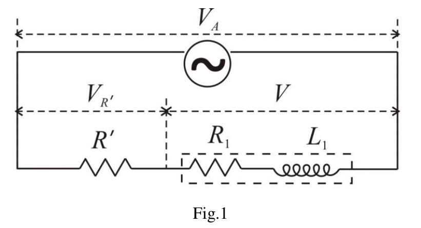
Fig.1

If the applied voltage across the series combination consisting of a known resistor $R^{\prime }$ with the coil is $V_A$, then an expression relating applied voltage $V_A$ to the voltage drops $V_{R^{\prime }}$ across $R^{\prime }$, $V$ across the coil and the angle $\theta$ is

V_A^2 = V_{R'}^2 + V^2 + 2V_{R'}V \cos \theta \tag{6}

All quantities except $\theta$ in Equation (6) are measurable.

Hence measuring the three voltages $V_A$, $V_{R^{\prime }}$ and $V$, and using Equations (4), (5) and (6), $\theta$, $R$ and $X$ can be determined. Knowing the frequency of the alternating current the value of $L$ can be calculated.

Alternatively, from Equations (4) and (6) we can express the value of $R$ in terms of the three measured voltages as

R = \left[\frac{R'}{2}\right]\left[\frac{V_A^2 - V^2}{V_{R'}^2} - 1\right] \tag{7}

The impedance $Z$ of the coil can be calculated using the formula $Z=\frac{V}{V_{R^{\prime }}}{R}^{\prime }$ and the value of $X$ could be obtained from

X = \sqrt{Z^2 - R^2} \tag{1A}

Coupled Circuits

The energy supplied by the power source to the primary can be dissipated partially in the primary and the remainder in other mutually coupled secondaries. When no mechanical work is done, the energy dissipation is only in resistances. The inductances store energy in the magnetic field associated with them. With current $I$ (rms value) the average stored energy in inductance $L$ is equal to $\frac{1}{2}L{I}^2$.

When a current flows in the secondary the emf induced due to it in the primary brings about change in the primary current. Seen from the primary side the effect is a consequence of change in the effective resistance and reactance of the primary coil and there is no need to know the parameters in the secondary circuit. The total energy dissipated in primary as well as secondary circuits appears as if it is dissipated in the effective primary resistance when seen from the primary side.

The effective values of resistance $R_{\mathrm{PE}}$ and inductance $L_{\mathrm{PE}}$ of primary can be related to a ‘reflected’ resistance $R_R$ and a ‘reflected’ inductance $L_R$ from the secondary side. The (average) power dissipated in the reflected resistance $R_R$ in the primary has to be equal to that in resistance $R_S$ in the secondary circuit. This gives

I_P^2 R_R = I_S^2 (R_S + R_L) \tag{8}

Similarly, we can relate the reflected inductance $L_R$ to the secondary inductance $L_S$ from

\frac{1}{2}L_R I_P^2 = \frac{1}{2}L_S I_S^2 \tag{9}

Considering the fact that the induced emf in the secondary due to an alternating primary current $I_P$ has magnitude equal to $\omega M{I}_P$ we can write the equation corresponding to Kirchhoff’s loop rule for the secondary in terms of rms values of primary and secondary currents as

\omega M I_P = I_S Z_S \tag{10}

where $Z_S$ is the impedance of the secondary circuit. When the secondary impedance is infinite the mutually induced emf appears as the voltage across the open ends of the secondary.

APPARATUS:

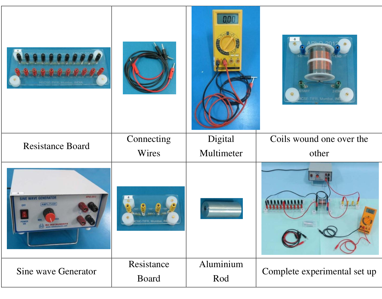
Resistance Board — Connecting Wires — Digital Multimeter — Coils wound one over the other — Sine wave Generator — Resistance Board — Aluminium Rod — Complete experimental set up

The apparatus provided for the experiment consists of the following.

1. A sine wave generator with output of about 10 V (rms) at 1000 Hz frequency
2. A digital multimeter (DMM) to be used as a voltmeter
3. A pair of coaxial coils wound one around the other on a cylindrical hollow piece of non magnetic non conducting bobbin
4. A piece of aluminium rod capable of fitting inside the bobbin
5. Two series of ten resistors mounted on an acrylic board: one consisting of 100 ohms resistors and the other of 10 ohms resistors with banana pin sockets
6. The required resistance for load $R_L$ or sampling resistance $R^{\prime }$ can be selected using this resistance board and connecting wire pieces. A separate acrylic board with resistance of 300 ohms is provided which can be used for sampling resistor when the other board is used for load resistance.
7. A set of five red and five black wires with banana pins at their ends (the pair of longer red and black wires is meant for use as DMM probes).

The output of the sine wave generator of frequency 1000 Hz is to be used as the alternating source voltage. Use the 20 V range of the DMM to measure rms ac voltages. The magnitudes of currents $I_P$ and $I_S$ when needed are to be calculated from the measured voltages across known values of $R^{\prime }$ in primary and $R_L$ in secondary respectively.

EXPERIMENT

PART 1: Determining Resistance and Inductance of a Coil with Air-core and Aluminium Core [3.4]

Connect coil 1 (with blue terminals) in series with a resistor $R^{\prime }$ (to be selected from the resistance board) across the output terminals of the sine wave generator. The sine wave generator will be on before you start your experiment for stabilization of its output. Do not turn it off. Keep the output voltage amplitude maximum. (The DMM should show the output about 10 V).

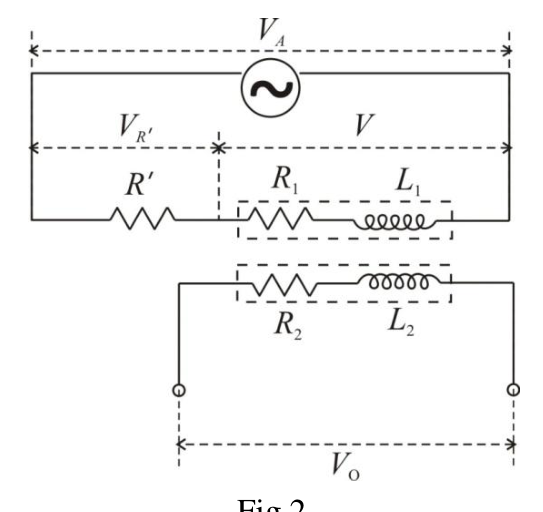
Fig.2

The ac output of the generator may have some asymmetry. In that case, the readings of the DMM will show slightly different readings, when the input polarities of the DMM are interchanged between ‘V/Ω’ to ‘com’. To correct for the error due to asymmetry repeat each reading by interchanging the polarity of the probes of the DMM and take the mean of the two readings.

Choose the value of R′ to obtain $V_{R^{\prime }}$ and $V$ approximately equal so that the systematic error in Z becomes negligible.

a) Measure the voltages $V_A$, $V_{R^{\prime }}$ and $V$ as well as $V_O$ across the terminals of the other coil. Determine the resistance $R_1$ and inductance $L_1$ of coil 1 (with blue terminals) and estimate the uncertainties in the values determined. (0.9)

b) Connect the other coil (coil 2 with green terminals), make the necessary measurements and determine $R_2$ and $L_2$. Evaluate the uncertainties in the values obtained. (0.9)

c) Now insert the piece of aluminium rod at the core of the coils and repeat the procedure to obtain the values of inductances $L_1\ast$ and resistance $R_1\ast$ and the uncertainties in them for coil1. (0.8)

d) Make necessary measurements and determine inductance $L_2\ast$ of coil 2 and resistance, $R_2\ast$ of coil 2 when it has an aluminium core. Estimate the uncertainties in the values. (0.8)

Note: Uncertainty calculations need not be done for parts 2, 3 and 4.

PART 2: Mutual Inductance and Coupling Constant [3.0]

f) Mutual inductance $M$ can be obtained from the readings of $V_{R^{\prime }}$ and $V_O$ (recorded in Part 1). Find the average values for air core as well as aluminium core coils. The relation between the mutual inductance and the self inductance of the coupled coils is given by $M=k(L_1{L}_2{)}^{1/2}$. Determine the value of $k$, the coupling coefficient in the two cases. (0.4)

g) Select coil 1 (with blue terminals) as primary and coil 2 (with green terminals) as secondary. Connect the primary in series with the sampling resistor $R^{\prime }=300$ ohms across the output terminals of the generator. Connect across the secondary the variable resistor $R_L$. The output voltage $V_O$ is to be measured across $R_L$. Change $R_L$ and measure the voltages $V_A$, $V_{R^{\prime }}$, $V$ and $V_O$ corresponding to each value of $R_L$. (0.8)

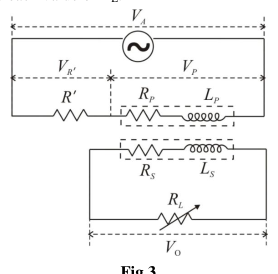
Fig.3

h) A linear graph can be plotted combining various terms appearing in Equation (10) written in expanded form. Write the linear expression for plotting a graph whose slope can be used to obtain the value of $M$ and intercept to obtain the value of secondary reactance $X_S$. (0.2)

i) Calculate the necessary quantities using data from (g) to plot the graph corresponding to the expression developed in the step (h) above. (0.9)

j) Plot the graph and obtain the values of $M$ and $X_S$. (0.7)

PART 3: Relations between Effective Primary Impedance and the Reflected Quantities from Secondary [2.4]

k) Use the data collected in Part 2 to determine the effective resistance $R_{\mathrm{PE}}$ of the primary corresponding to each value of $R_L$ in secondary. (0.6)

l) Use the data of Part 2 to calculate the values of reflected resistance $R_R$ as defined in Equation (8) and of reflected reactance $X_R$ referring Equation (9) corresponding to the values of $R_L$. (0.6)

m) Plot graph of $X_{\mathrm{PE}}$ against $X_R$. Taking into consideration the likely uncertainties of the quantities plotted write down the equation giving the relationship between the effective primary reactance and the reflected reactance. (0.6)

n) Represent graphically the relation between $R_R$ and $R_L$ over the range of study and find the value of $R_L$ for which the reflected resistance attains a maximum. If needed, take some more observations to supplement the observations in Part 2 for locating the point with greater precision. (0.6)

PART 4: Eddy Current Effects [1.2]

o) A model based on the analysis of the data in Part 3 suggests how to estimate the ratio of inductance and resistance seen by the eddy currents set up in the core of a coil connected to a power source.

The analysis of the data of Part 2(i) and (j) should show that $R_{\mathrm{PE}}=R_P+R_R$. The relation between $X_{\mathrm{PE}}$ and $X_R$ is obtained from Part 3(m).

Refer to the data collected in Part 1(c) and Part 2 respectively to determine the ratio of inductance and resistance as seen by eddy currents in the aluminium core when the power supply is connected to coil 1 and coil 2 respectively. (0.8)

p) Connect the coils as in Part 2 Fig.3 and insert the piece of aluminium rod into the core in the aluminium core. The relation between $R_{\mathrm{PE}}$ and $R_R$ is obtained from Part 3(m).

Set $R^{\prime }=300$ ohms and $R_L=1000$ ohms. Adjust the magnitude of $V_A$ equal to 9.0 V. Make the necessary measurements and calculate the power dissipation due to the eddy currents in the aluminium core. (0.4)

Fonte: Testo (PDF) — p.1 Topic: Electromagnetic Induction, Circuits Metodi: Faraday’s Law of Induction, Kirchhoff’s Laws, Experimental Data Analysis, Graph Linearization Competenze: Experimental Data Analysis, Measurement & Instrumentation, Error Propagation, Graph Linearization Objects: Coil, Resistor, Wire

Induzione elettromagnetica

La tecnica moderna di prova di corrente a corrente a sciapo utilizzata per rilevare difetti sotto le superfici di oggetti metallici si basa sui principi dell’induzione elettromagnetica. Le correnti circolanti indotte nei corpi conduttori a causa del flusso magnetico in variazione nella regione in cui si trovano sono chiamate correnti di eddy. I difetti sono rilevati osservando i cambiamenti nella resistenza e nell’inductanza di una bobina che porta corrente alternata quando viene tenuta vicino alla superficie dell’oggetto.

A meno che il nucleo del solenoide non contenga materiale ferromagnetico, il flusso magnetico $\varphi$ è proporzionale alla corrente $i$. La costante di proporzionalità è chiamata auto-induzione della bobina e è rappresentata dalla lettera $L$. L’emf auto-indotto in una bobina con induttanza $L$ è:

di cui $-L\frac{di}{dt}$.

In un sistema di circuiti abbinati con corrente $i_1$ in un circuito il flusso magnetico collegato a esso è dato da

$\varphi =L_1{i}_1+M_{12}{i}_2$

Where $L_1$ is the self inductance of that circuit and $M_{12}$ is the mutual inductance of the coupled system. Un’equazione simile vale per l’inverso, con $M_{12}=M_{21}$.

Circuito L-R

Una corrente sinusoidale in alternazione con frequenza angolare $\omega$ che scorre attraverso una combinazione di serie di resistenza $R$ e di induttanza $L$ produce una caduta di tensione attraverso la combinazione.

Se rappresentiamo la corrente con $i=I_0\sin \omega t$, la caduta di tensione attraverso la resistenza è uguale a $I_{0}R\sin \omega t$ e attraverso l’inductanza è $I_0\omega L\cos \omega t$. Possiamo combinarli per ottenere la tensione attraverso la combinazione $R$-$L$. La quantità $\omega L$ è chiamata reattanza induttiva e è rappresentata dal simbolo $X$. Si può facilmente dimostrare che la tensione attraverso la bobina è uguale a $I_{0}Z\sin (\omega t+\theta )$, dove

Z = \sqrt{R^2 + X^2} \tag{1}

e

\theta = \tan^{-1}\!\left(\frac{X}{R}\right) \tag{2}

La tensione alternata e la corrente variano continuamente sia nella magnitudine che nella polarità nel corso del tempo, ma i valori rms di queste quantità calcolate nel corso di un ciclo sono indipendenti dal tempo e la relazione $V=IZ$, dove entrambi $V$ e $I$ rappresentano i valori rms, è analoga alla legge di Ohm. Da questo vediamo che

V^2 = (IR)^2 + (IX)^2 \tag{3}

*(Nota:- Il concetto di resistenza è fondamentalmente correlato alla dissipazione di energia elettrica e il valore di resistenza di una bobina nel circuito ac può essere diverso dal suo valore determinato applicando la legge di Ohm con correnti dc.) *

Quando ci sono ulteriori resistenze e/o inductanze in serie con la bobina, possiamo ancora considerare il calo di tensione attraverso la combinazione come uguale alla radice quadrata della somma dei quadrati di calo di tensione attraverso la resistenza totale e attraverso l’inductanza totale.

Misura dell’induttura e della resistenza di una bobina

Per la misurazione della corrente e della tensione alternate, generalmente vengono segnalati i valori rms. Dalle equazioni (2) e (3) otteniamo

V \cos \theta = IR \tag{4}

e

V \sin \theta = IX \tag{5}

Per ottenere i valori $R$ e $L$ della bobina possiamo utilizzare le equazioni di cui sopra. Si possono misurare la tensione $V$ e la corrente $I$. Ma essendo ci sono tre quantità sconosciute $\theta$, $R$ e $X$ abbiamo bisogno di un’altra equazione.

Fig.1

Se la tensione applicata attraverso la combinazione di serie costituita da una resistenza nota $R^{\prime }$ con la bobina è $V_A$, allora un’espressione relativa alla tensione applicata $V_A$ alla caduta di tensione $V_{R^{\prime }}$ attraverso $R^{\prime }$, $V$ attraverso la bobina e l’angolo $\theta$ è

V_A^2 = V_{R'}^2 + V^2 + 2V_{R'}V \cos \theta \tag{6}

Tutte le quantità, tranne $\theta$ nell’equazione (6), sono misurabili.

Si possono quindi determinare le tre tensioni $V_A$, $V_{R^{\prime }}$ e $V$, utilizzando le equazioni (4), (5) e (6), $\theta$, $R$ e $X$. Con la conoscenza della frequenza della corrente alternata si può calcolare il valore di $L$.

In alternativa, dalle equazioni (4) e (6) possiamo esprimere il valore di $R$ in termini di tre tensioni misurate come

R = \left[\frac{R'}{2}\right]\left[\frac{V_A^2 - V^2}{V_{R'}^2} - 1\right] \tag{7}

L’impedenza $Z$ della bobina può essere calcolata con la formula $Z=\frac{V}{V_{R^{\prime }}}{R}^{\prime }$ e il valore di $X$ può essere ottenuto da

X = \sqrt{Z^2 - R^2} \tag{1A}

Circuiti accoppiati

L’energia fornita dalla fonte di alimentazione al primario può essere dissipata in parte nel primario e il resto in altri secondari reciprocamente accoppiati. Quando non si fa alcun lavoro meccanico, la dissipazione dell’energia è solo in resistenze. Le inductance conservano energia nel campo magnetico associato a loro. Con corrente $I$ (valore rms) l’energia media immagazzinata in inductanza $L$ è uguale a $\frac{1}{2}L{I}^2$.

Quando una corrente scorre nel secondario l’emf indotto a causa di essa nel primario provoca un cambiamento nel corrente primaria. Visto dal lato primario, l’effetto è una conseguenza di un cambiamento della resistenza effettiva e della reattanza della bobina primaria e non è necessario conoscere i parametri del circuito secondario. L’energia totale dissipata nei circuiti primari e secondari appare come se fosse dissipata nella resistenza primaria effettiva quando vista dal lato primario.

I valori effettivi di resistenza $R_{\mathrm{PE}}$ e di inductanza $L_{\mathrm{PE}}$ della resistenza primaria possono essere correlati a una resistenza $R_R$ “riflessa” e ad una inductanza $L_R$ “riflessa” dal lato secondario. La potenza (media) dissipata nella resistenza riflessa $R_R$ nel primo deve essere uguale a quella della resistenza $R_S$ nel circuito secondario. Questo dà

I_P^2 R_R = I_S^2 (R_S + R_L) \tag{8}

Allo stesso modo, possiamo collegare l’induttanza riflessa $L_R$ all’induttanza secondaria $L_S$ da

\frac{1}{2}L_R I_P^2 = \frac{1}{2}L_S I_S^2 \tag{9}

Considerando il fatto che l’emf indotto nel secondario a causa di una corrente primaria alternata $I_P$ ha magnitudine uguale a $\omega M{I}_P$ possiamo scrivere l’equazione corrispondente alla regola di loop di Kirchhoff per il secondario in termini di valori rms di correnti primarie e secondarie come

\omega M I_P = I_S Z_S \tag{10}

dove $Z_S$ è l’impedenza del circuito secondario. Quando l’impedenza secondaria è infinita, l’emf indotto reciprocamente appare come la tensione attraverso le estremità aperte del secondario.

apparecchiatura:

Tavola di resistenza Fonte di connessione Multimetro digitale Coil ferita l’una sull’altra Generatore d’onda di sinte Tavola di resistenza Rod di alluminio Completa installazione sperimentale

L’apparecchio fornito per l’esperimento è costituito dai seguenti elementi:

1. Generatore di onde sinusoide con uscita di circa 10 V (rms) a frequenza 1000 Hz
2. Un multimetro digitale (DMM) da utilizzare come voltmeter
3. Un paio di bobine coassiali rotate l’una intorno all’altra su un pezzo vuoto cilindrico di bobina non magnetica non conduttrice
4. Fabbrica di canna di alluminio che può essere montata all’interno della bobina
5. Due serie di dieci resistori montati su una tavola acrilica: uno composto da resistori da 100 ohms e l’altro da resistori da 10 ohms con prese di pin di banana
6. La resistenza richiesta per il carico $R_L$ o la resistenza al campionamento $R^{\prime }$ può essere selezionata utilizzando questa scheda di resistenza e i pezzi di filo di connessione. Si dispone di una tabella acrilica separata con una resistenza di 300 ohm che può essere utilizzata per la resistenza al campionamento quando l’altra tabella viene utilizzata per la resistenza al carico.
7. Un insieme di cinque fili rossi e cinque neri con pinci di banana alle estremità (il paio di fili rossi e neri più lunghi è destinato all’uso come sonde DMM).

La potenza di uscita del generatore di onde sinusoide di frequenza 1000 Hz deve essere utilizzata come tensione sorgente alternata. Utilizzare la gamma di 20 V del DMM per misurare le tensioni ac. Le magnitudini delle correnti $I_P$ e $I_S$, quando necessario, devono essere calcolate a partire dalle tensioni misurate attraverso i valori noti di $R^{\prime }$ in primario e $R_L$ in secondario rispettivamente.

# esperimento

PARTE 1: Determinazione della resistenza e dell’induzione di una bobina con nucleo di aria e nucleo di alluminio [3.4]

Connettere la bobina 1 (con terminali blu) in serie con una resistenza $R^{\prime }$ (a selezionare dalla scheda di resistenza) attraverso i terminali di uscita del generatore di onde sinusoide. Il generatore di onde sinusoide sarà acceso prima di iniziare l’esperimento per stabilizzare la sua uscita. Non spegnere. Tenere l’ampiezza della tensione di uscita al massimo. (Il DMM dovrebbe mostrare la potenza di circa 10 V).

Fig.2

La produzione di ac del generatore può avere una certa asimmetria. In tal caso, le letture del DMM mostreranno letture leggermente diverse, quando le polarità di ingresso del DMM sono scambiate tra “V/Ω” e “com”. Per correggere l’errore dovuto all’asimmetria, ripetere ogni lettura scambiando la polarità delle sonde del DMM e prendere la media delle due letture.

Scelta il valore di R′ per ottenere $V_{R^{\prime }}$ e $V$ approssimativamente uguali in modo che l’errore sistematico in Z diventi trascurabile.

**a) ** Misurare le tensioni $V_A$, $V_{R^{\prime }}$ e $V$ nonché $V_O$ attraverso i terminali dell’altra bobina. Determinare la resistenza $R_1$ e l’inductanza $L_1$ della bobina 1 (con terminali blu) e stimare le incertezze nei valori determinati. (0.9)

**b) ** Collegare l’altra bobina ( bobina 2 con terminali verdi), effettuare le misure necessarie e determinare $R_2$ e $L_2$. Valutare le incertezze dei valori ottenuti. (0.9)

**c) ** Ora inserire il pezzo di canna di alluminio nel nucleo delle bobine e ripetere la procedura per ottenere i valori delle induttanze $L_1\ast$ e della resistenza $R_1\ast$ e le incertezze presenti per la bobina1. (0.8)

**d) ** Fare le misure necessarie e determinare l’induttanza $L_2\ast$ della bobina 2 e la resistenza $R_2\ast$ della bobina 2 quando ha un nucleo di alluminio. Estimare le incertezze dei valori. (0.8)

Nota: non è necessario effettuare calcoli di incertezza per le parti 2, 3 e 4.

PARTE 2: Induttanza reciproca e costante di accoppiamento [3.0]

f) ** L’ induttanza reciproca $M$ può essere ottenuta dalle letture di $V_{R^{\prime }}$ e $V_O$ (registrate in ** Parte 1). Trova i valori medi per il nucleo d’aria e per le bobine di nucleo di alluminio. Il rapporto tra l’induzione reciproca e l’autoinduzione delle bobine accoppiate è dato da $M=k(L_1{L}_2{)}^{1/2}$. Determinare il valore di $k$, il coefficiente di accoppiamento nei due casi. (0.4)

**g) ** Selezionare la bobina 1 (con terminali blu) come primaria e la bobina 2 (con terminali verdi) come secondaria. Connettere la prima in serie con la resistenza di campionamento $R^{\prime }=300$ ohms attraverso i terminali di uscita del generatore. Collegare attraverso il secondario la resistenza variabile $R_L$. La tensione di uscita $V_O$ deve essere misurata su $R_L$. Cambiare $R_L$ e misurare le tensioni $V_A$, $V_{R^{\prime }}$, $V$ e $V_O$ corrispondenti a ciascun valore di $R_L$. (0.8)

Fig.3

**h) ** Si può disegnare un grafico lineare che combina vari termini che appaiono nell’Equazione (10) scritti in forma ampliata. Scrivere l’espressione lineare per tracciare un grafico la cui pendenza ** può essere utilizzata per ottenere il valore di $M$ e intercettare per ottenere il valore di reazione secondaria $X_S$. (0.2)

**i) ** Calcolare le quantità necessarie utilizzando i dati di **(g) ** per tracciare il grafico corrispondente all’espressione sviluppata nel passaggio **(h) ** di cui sopra. (0.9)

**j) ** Tracciare il grafico e ottenere i valori di $M$ e $X_S$. (0.7)

PARTE 3: Relazioni tra l’impedenza primaria effettiva e le quantità riflesse dal secondario [2.4]

**k) ** Utilizzare i dati raccolti nella parte 2 per determinare la resistenza effettiva $R_{\mathrm{PE}}$ della prima corrispondente a ogni valore di $R_L$ nella seconda. (0.6)

**l) ** Utilizzare i dati di Part 2 per calcolare i valori della resistenza riflessa $R_R$ come definiti nell’Equazione (8) e della reattività riflessa $X_R$ riferendosi all’Equazione (9) corrispondenti ai valori di $R_L$. (0.6)

**m) ** Grafico di trama di $X_{\mathrm{PE}}$ contro $X_R$. Tenendo conto delle probabili incertezze delle quantità tracciate, scrivere l’equazione che fornisce la relazione tra la reazione primaria effettiva e la reazione riflessa. (0.6)

**n) ** Rappresenta graficamente la relazione tra $R_R$ e $R_L$ nel raggio di studio e trova il valore di $R_L$ per il quale la resistenza riflessa raggiunge il massimo. If needed, take some more observations to supplement the observations in Part 2 for locating the point with greater precision. (0.6)

PARTE 4: Effetti Eddy Current [1.2]

o) A model based on the analysis of the data in Part 3 suggests how to estimate the ratio of inductance and resistance seen by the eddy currents set up in the core of a coil connected to a power source.

L’analisi dei dati di **parte 2 ((i) ** e **(j) ** dovrebbe dimostrare che $R_{\mathrm{PE}}=R_P+R_R$. Il rapporto tra $X_{\mathrm{PE}}$ e $X_R$ è ottenuto da **Parte 3(m) **.

Refer to the data collected in Part 1(c) and Part 2 respectively to determine the ratio of inductance and resistance as seen by eddy currents in the aluminium core when the power supply is connected to coil 1 and coil 2 respectively. (0.8)

p) Connect the coils as in Part 2 Fig.3 and insert the piece of aluminium rod into the core in the aluminium core. Il rapporto tra $R_{\mathrm{PE}}$ e $R_R$ è ottenuto da **Parte 3(m) **.

Impostare $R^{\prime }=300$ ohms e $R_L=1000$ ohms. Raggiustare la magnitudine di $V_A$ pari a 9,0 V. Fare le misure necessarie e calcolare la dissipazione di potenza dovuta alle correnti di artigliamento nel nucleo di alluminio. (0.4)

Fonte: Testo (PDF) — p.1 Topic: Electromagnetic Induction, Circuits Metodi: Faraday’s Law of Induction, Kirchhoff’s Laws, Experimental Data Analysis, Graph Linearization Competenze: Experimental Data Analysis, Measurement & Instrumentation, Error Propagation, Graph Linearization Objects: Coil, Resistor, Wire