APhO 2012 — Teorica

The Drag on a Falling Magnet

A clear and detailed discussion on eddy currents was first provided by the British physicist Sir James H. Jeans (1877–1946) in his celebrated book The mathematical theory of electricity and magnetism (1925). The present problem is based on electricity and magnetism.

A small size magnet with dipole moment of magnitude $p$ and mass $m$ is dropped through a very long vertically held non-magnetic metallic tube as shown in Fig. (1) (figure is not to scale). In general the fall is governed by

m\ddot{z} = mg - k\dot{z} \tag{1}

Here $g$ is the acceleration due to gravity. Note that the damping parameter $k$ is due to the generation of eddy currents in the tube.

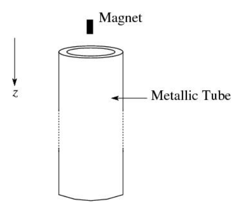Figure 1

I.1 Obtain the terminal velocity ($v_T$) of the magnet. [0.5 point]

I.2 Obtain $z(t)$, i.e. position of the magnet at time $t$. Take $v(t=0)=0$ and $z(t=0)=0$. [1.0 point]

We shall attempt to understand the dynamics of the fall. In order to do this we consider in part (I.3) – part (I.8) a simplified problem of the magnet falling axially towards a fixed non-magnetic metallic ring of radius $a$, resistance $R$ and inductance $L$ as shown in Fig. (2). In this problem, we shall ignore radiation effects.

In our case it is convenient to change the reference coordinates to a set of cylindrical ones $(\rho ,\phi ,z)$ as shown in Fig. (2) where $z$-axis is the ring axis, the magnet is initially at rest at the origin and the center of the ring is at distance $z_0$ from the origin. Cartesian axes $(x,y,z)$ are also shown in the figure. The magnet has dipole moment $p$ in the positive $z$ direction ($\vec{p}=p\hat{k}$) where $\hat{k}$ is unit vector in $z$ direction. We will assume that during the fall, magnetic moment remains in the same direction. The axial component ($B_z$) and radial component ($B_{\rho }$) of the magnetic field at an arbitrary point $(\rho ,\phi ,z)$ when the magnet is at the origin are given by

$B_z=\frac{{\mu }_0}{4\pi }\frac{p}{({\rho }^2+z^2{)}^{3/2}}\left[\frac{3z^2}{{\rho }^2+z^2}-1\right]$

$B_{\rho }=\frac{{\mu }_0}{4\pi }\frac{3pz\rho }{({\rho }^2+z^2{)}^{5/2}}$

where ${\mu }_0$ is the permeability of free space.

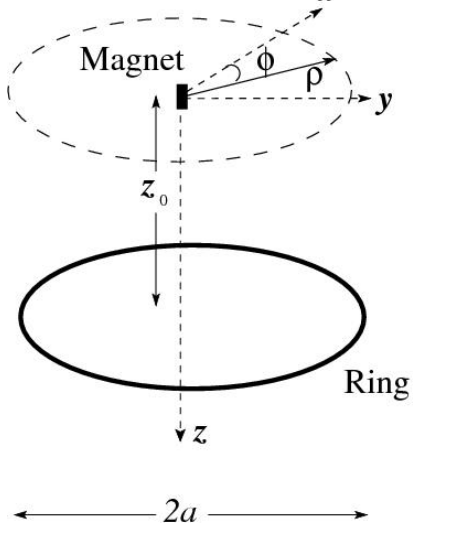Figure 2

I.3 Let the instantaneous speed of the magnet be $v$. Obtain the magnitude of the induced emf ($e_i$) in the ring. [1.5 points]

I.4 This emf will give rise to an induced current ($i$) in the ring. Obtain the magnitude of the instantaneous electromagnetic force ($f_{em}$) on the ring in terms of $i$. [1.0 point]

I.5 What is the magnitude of the force on the magnet due to this ring? [0.5 point]

I.6 Express the emf in the ring in terms of $L$, $R$ and $i$. Do not solve for $i$. [0.5 point]

I.7 As the magnet falls it loses gravitational potential energy. Identify the three main forms of energy into which the gravitational potential energy is converted and write down the expressions you would use to calculate each of the three contributions. [1.0 point]

I.8 Does the magnetic field of the magnet do any work in this process? Tick in the appropriate box. [0.5 point]

Next we will estimate the damping parameter $k$ due to the pipe (see Eq. (1)). Take an infinitely long pipe with radius $a$, small thickness $w$, and electrical conductivity $\sigma$. For this and later part, we take inductance of the pipe to be negligible. It would help if you considered the pipe to be made of many rings each of height $\Delta z^{\prime }$, radius $a$, small thickness $w$ and electrical conductivity $\sigma$ (see Fig. (3)). For simplicity, the two ends of the pipe are at $z=-\infty$ and at $z=\infty$, respectively.

I.9 Obtain the resistance of an individual ring. [0.5 point]

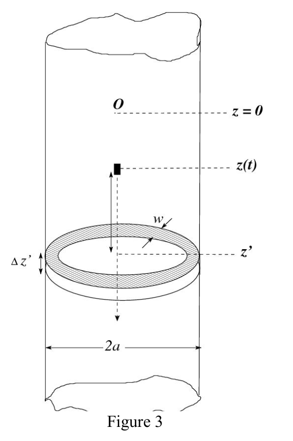Figure 3

I.10 Obtain the damping parameter $k$ due to the entire pipe in terms of $p$, $\sigma$ and geometrical parameters of the ring. Since each ring is very thin, you may take magnetic field to be constant over the thickness of the ring and equal to $B_{\rho }(\rho =a)$. Assume that at an instant $t$, the magnet has a coordinate $z(t)$ with an instantaneous speed $\dot{z}$. You should leave your answer in terms of a dimensionless integral $I$, involving a dimensionless variable $u=(z-z^{\prime })/a$. [2.0 points]

I.11 Assume that the damping constant $k$ depends on the following

$k=f({\mu }_0,p,R_0,a)$

where $R_0$ is the effective resistance of a long pipe. Use dimensional analysis to obtain an expression for $k$. Take the dimensionless constant to be unity. [1.0 point]

The following integral may be useful:

$\int \frac{udu}{(u^2+a^2{)}^n}=\frac{1}{2}\frac{(a^2+u^2{)}^{1-n}}{1-n}+\text{Constant}(n>1)$

Fonte: Testo (PDF) — p.1

Topic: Electromagnetic Induction, Electromagnetism Metodi: Faraday’s Law of Induction, Lenz’s Law, Differential Equations, Dimensional Analysis Competenze: Mathematical Modeling, Physical Reasoning Objects: Magnetic Dipole, Tube, Magnet

Il trascinamento su un magnete cadente

Una discussione chiara e dettagliata sulle correnti eddy fu fornita per la prima volta dal fisico britannico Sir James H. Jeans (18771946) nel suo celebre libro La teoria matematica dell’elettricità e del magnetismo (1925). Il problema attuale si basa sull’elettricità e sul magnetismo.

Un magnete di piccola dimensione con momento di dipole di magnitudo $p$ e massa $m$ viene trasmesso attraverso un tubo metallico non magnetico tenuto verticalmente molto lungo come mostrato nella figura. (1) (la figura non è in scala). In generale, l’autunno è regolato da

m\ddot{z} = mg - k\dot{z} \tag{1}

Qui $g$ è l’accelerazione dovuta alla gravità. Si noti che il parametro di ammortizzazione $k$ è dovuto alla generazione di correnti di scarico nel tubo.

Figura 1

I.1 Ottieni la velocità terminale ($v_T$) del magnete. [0,5 punto]

**I.2 ** Ottenere $z(t)$, ovvero posizione del magnete al tempo $t$. Prendete $v(t=0)=0$ e $z(t=0)=0$. [1,0 punto]

Cercheremo di capire la dinamica della caduta. Per fare questo consideriamo in parte (I.3) parte (I.8) un problema semplificato del magnete che cade assiale verso un anello metallico non magneto fisso di raggio $a$, resistenza $R$ e inductanza $L$ come mostrato nella figura. (2). In questo problema, ignoriamo gli effetti delle radiazioni.

Nel nostro caso è conveniente modificare le coordinate di riferimento in un insieme di quelle cilindriche $(\rho ,\phi ,z)$ come mostrato nella figura. (2) se l’asse $z$ è l’asse dell’anello, il magnete è inizialmente a riposo all’origine e il centro dell’anello è a distanza $z_0$ dall’origine. Anche le assi cartesiane $(x,y,z)$ sono illustrate nella figura. Il magnete ha il momento di dipole $p$ nella direzione positiva $z$ ($\vec{p}=p\hat{k}$) dove $\hat{k}$ è vettore unitario nella direzione $z$. Supponiamo che durante l’autunno il momento magnetico rimanga nella stessa direzione. La componente asiale ($B_z$) e la componente radiale ($B_{\rho }$) del campo magnetico in un punto arbitrario $(\rho ,\phi ,z)$ quando il magnete è all’origine sono indicate da:

$B_z=\frac{{\mu }_0}{4\pi }\frac{p}{({\rho }^2+z^2{)}^{3/2}}\left[\frac{3z^2}{{\rho }^2+z^2}-1\right]$

$B_{\rho }=\frac{{\mu }_0}{4\pi }\frac{3pz\rho }{({\rho }^2+z^2{)}^{5/2}}$

in cui ${\mu }_0$ è la permeabilità dello spazio libero.

Figura 2

**I.3 ** La velocità istantanea del magnete deve essere $v$. Ottenere la magnitudine dell’emf indotto ($e_i$) nell’anello. [1,5 punti]

**I.4 ** Questa emf darà luogo a una corrente indotta ($i$) nell’anello. Ottenere la grandezza della forza elettromagnetica istantanea ($f_{em}$) sull’anello in termini di $i$. [1,0 punto]

Qual è la grandezza della forza sul magnete dovuta a questo anello? [0,5 punto]

**I.6 ** Esprimere l’emf nell’anello in termini di $L$, $R$ e $i$. Non risolvere per $i$. [0,5 punto]

Quando il magnete cade perde energia gravitazionale potenziale. Identifica le tre principali forme di energia in cui si converte l’energia potenziale gravitazionale e scrivi le espressioni che utilizzerai per calcolare ciascuno dei tre contributi. [1,0 punto]

Il campo magnetico del magnete svolge un qualsiasi lavoro in questo processo? - Metti la casella appropriata. [0,5 punto]

In seguito stimeremo il parametro di ammortizzazione $k$ dovuto al tubo (vedere Eq. (1)). Prendi un tubo infinitamente lungo con raggio $a$, spessore $w$ e conduttività elettrica $\sigma$. Per questa e la parte successiva, la inductanza della tubazione è trascurabile. Sarebbe utile se considerasse che il tubo sia costituito da molti anelli, ognuno di altezza $\Delta z^{\prime }$, raggio $a$, spessore $w$ e conduttività elettrica $\sigma$ (vedere figura 1. (3)). Per semplicità, le due estremità del tubo sono rispettivamente $z=-\infty$ e $z=\infty$.

**I.9 ** Ottenere la resistenza di un singolo anello. [0,5 punto]

Figura 3

I.10 Ottieni il parametro di ammortizzazione $k$ dovuto a tutto il tubo in termini di $p$, $\sigma$ e parametri geometrici dell’anello. Poiché ogni anello è molto sottile, si può prendere un campo magnetico per essere costante sullo spessore dell’anello ed è uguale a $B_{\rho }(\rho =a)$. Supponiamo che ad un istante $t$, il magnete abbia una coordinata $z(t)$ con una velocità istantanea $\dot{z}$. La risposta deve essere presentata in termini di integrale senza dimensioni $I$, che coinvolge una variabile senza dimensioni $u=(z-z^{\prime })/a$. [2,0 punti]

I.11 Supponiamo che la costante di ammortizzazione $k$ dipenda da quanto segue:

$k=f({\mu }_0,p,R_0,a)$

dove $R_0$ è la resistenza effettiva di un tubo lungo. Utilizzare l’analisi dimensionale per ottenere un’espressione per $k$. Prendi la costante senza dimensioni per essere unità. [1,0 punto]

La seguente integrale può essere utile:

$\int \frac{udu}{(u^2+a^2{)}^n}=\frac{1}{2}\frac{(a^2+u^2{)}^{1-n}}{1-n}+\text{Constant}(n>1)$

Fonte: Testo (PDF) — p.1

Topic: Electromagnetic Induction, Electromagnetism Metodi: Faraday’s Law of Induction, Lenz’s Law, Differential Equations, Dimensional Analysis Competenze: Mathematical Modeling, Physical Reasoning Objects: Magnetic Dipole, Tube, Magnet

Chandrasekhar Limit

In a famous work carried out in 1930, the Indian Physicist Prof Subrahmanyan Chandrasekhar (1910–1995) studied the stability of stars. The problem will help you to construct a simplified version of his analysis.

You may find the following symbols and values useful.

Quantity	Symbol and value
Speed of light in vacuum	$c=3.00\times 10^8\mathrm{m}{\mathrm{s}}^{-1}$
Planck’s constant	$h=6.63\times 10^{-34}\mathrm{J}\mathrm{s}$
Universal constant of Gravitation	$G=6.67\times 10^{-11}\mathrm{N}{\mathrm{m}}^2\mathrm{k}{\mathrm{g}}^{-2}$
Rest mass of electron	$m_e=9.11\times 10^{-31}\mathrm{kg}$
Rest mass of proton	$m_p=1.67\times 10^{-27}\mathrm{kg}$

II.1 Consider a spherical star of uniform density, radius $R$ and mass $M$. Derive an expression for its gravitational potential energy ($E_G$) due to its own gravitational field (gravitational self energy). [1.0 point]

II.2 We assume that the star is made up of only hydrogen and that all the hydrogen is in ionized form. We consider the situation when the star’s energy production due to nuclear fusion has stopped. Electrons obey the Pauli exclusion principle and their total energy can be computed using quantum statistics. You may take this total electronic energy (ignoring the protonic energy) to be

$E_e=\frac{{\hslash }^2{\pi }^3}{10m_e{4}^{2/3}}{\left(\frac{3}{\pi }\right)}^{7/3}\frac{N_e^{5/3}}{R^2}$

where $N_e$ is the total number of electrons and $\hslash =h/2\pi$. Obtain the equilibrium condition of the star relating its radius ($R_{wd}$) to its mass. This radius is called the ‘White Dwarf’ radius. [2.0 points]

II.3 Numerically evaluate $R_{wd}$ given that mass of the star is the same as the solar mass ($M_S=2.00\times 10^{30}\mathrm{kg}$). [1.5 points]

II.4 Assuming that the electron distribution is homogeneous, obtain an order of magnitude estimation of the average separation ($r_{sep}$) between electrons if the radius of the star is $R_{wd}$ as obtained in part (II.3). [1.0 point]

II.5 Let us estimate the speed of electrons. For this purpose, assume each electron to form a standing wave in a one-dimensional box of length $r_{sep}$. Estimate the speed of electron ($v$) in the lowest energy state using de-Broglie hypothesis. [1.0 point]

II.6 Consider now a modification of the analysis in part (II.2). If we take electrons in the ultrarelativistic limit ($E=pc$), a similar analysis yields

$E_e^{rel}=\frac{{\pi }^2}{4^{4/3}}{\left(\frac{3}{\pi }\right)}^{5/3}\frac{\hslash c}{R}{N}_e^{4/3}$

Obtain the expression for the mass for which, the star can be in equilibrium in terms of the constants provided at the beginning of the question. We call this the critical mass ($M_c$). [1.5 points]

II.7 If the mass $M$ of the star is greater than the critical mass $M_c$ obtained in part (II.6), state whether the star will expand or contract. Tick in appropriate box. [0.5 point]

II.8 Calculate a numerical estimate of this critical mass in units of solar mass ($M_S$). (Note: Your answer may differ from Chandrasekhar’s famous result because of the approximations made in this analysis) [1.5 points]

Fonte: Testo (PDF) — p.1

Topic: Astrophysics, Modern-Quantum Physics Metodi: Newton’s Law of Gravitation, Energy Conservation Method, de Broglie Relation, Order-of-Magnitude Estimation Competenze: Estimation & Approximation, Mathematical Modeling Objects: Star, Electron

Chandrasekhar Limit

In un famoso lavoro svolto nel 1930, il fisico indiano Prof Subrahmanyan Chandrasekhar (1910-1995) studiò la stabilità delle stelle. Il problema ti aiuterà a costruire una versione semplificata della sua analisi.

Potreste trovare utili i seguenti simboli e valori.

Quantità, simbolo e valore. | --- | --- | | Speed of light in vacuum | $c=3.00\times 10^8\mathrm{m}{\mathrm{s}}^{-1}$ | | Planck’s constant | $h=6.63\times 10^{-34}\mathrm{J}\mathrm{s}$ | | Universal constant of Gravitation | $G=6.67\times 10^{-11}\mathrm{N}{\mathrm{m}}^2\mathrm{k}{\mathrm{g}}^{-2}$ | | Rest mass of electron | $m_e=9.11\times 10^{-31}\mathrm{kg}$ | | Rest mass of proton | $m_p=1.67\times 10^{-27}\mathrm{kg}$ |

**II.1 ** Considerate una stella sferica di densità uniforme, raggio $R$ e massa $M$. Derivare un’espressione per la sua energia potenziale gravitazionale ($E_G$) dovuta al suo campo gravitazionale (energia gravitazionale di sé). [1,0 punto]

II.2 We assume that the star is made up of only hydrogen and that all the hydrogen is in ionized form. Consideramo la situazione in cui la produzione di energia della stella a causa della fusione nucleare è stata interrotta. Gli elettroni obbediscono al principio di esclusione di Pauli e la loro energia totale può essere calcolata utilizzando statistiche quantistiche. Si può prendere questa energia elettronica totale (ignorando l’ energia protonica) per essere

$E_e=\frac{{\hslash }^2{\pi }^3}{10m_e{4}^{2/3}}{\left(\frac{3}{\pi }\right)}^{7/3}\frac{N_e^{5/3}}{R^2}$

dove $N_e$ è il numero totale di elettroni e $\hslash =h/2\pi$. Ottenere la condizione di equilibrio della stella che relaziona il suo raggio ($R_{wd}$) alla sua massa. Questo raggio è chiamato raggio “Nano Bianco”. [2,0 punti]

II.3 Valutare numericamente $R_{wd}$ dato che la massa della stella è la stessa della massa solare ($M_S=2.00\times 10^{30}\mathrm{kg}$). [1,5 punti]

II.4 Supponendo che la distribuzione degli elettroni sia omogenea, si ottiene un’ordine di stima di grandezza della separazione media ($r_{sep}$) tra gli elettroni se il raggio della stella è $R_{wd}$ come ottenuto nella parte (II.3). [1,0 punto]

II.5 Let us estimate the speed of electrons. Per questo scopo, supponiamo che ogni elettrone formi un’onda in piedi in una scatola unidimensionale di lunghezza $r_{sep}$. Estimare la velocità di elettrone ($v$) nello stato di energia più basso utilizzando l’ipotesi de-Broglie. [1,0 punto]

**II.6 ** Considera ora una modifica dell’analisi in parte (II.2). Se prendiamo gli elettroni nel limite ultrarellativistico ($E=pc$), una analisi simile produce

$E_e^{rel}=\frac{{\pi }^2}{4^{4/3}}{\left(\frac{3}{\pi }\right)}^{5/3}\frac{\hslash c}{R}{N}_e^{4/3}$

Ottenere l’espressione per la massa per la quale, la stella può essere in equilibrio in termini di costanti forniti all’inizio della domanda. Questo è chiamato massa critica ($M_c$). [1,5 punti]

II.7 If the mass $M$ of the star is greater than the critical mass $M_c$ obtained in part (II.6), state whether the star will expand or contract. - Metti la casella appropriata. [0,5 punto]

II.8 Calcolare una stima numerica di questa massa critica in unità di massa solare ($M_S$). (Nota: la tua risposta può differire dal famoso risultato di Chandrasekhar a causa delle approssimazioni fatte in questa analisi) [1,5 punti]

Fonte: Testo (PDF) — p.1

Topic: Astrophysics, Modern-Quantum Physics Metodi: Newton’s Law of Gravitation, Energy Conservation Method, de Broglie Relation, Order-of-Magnitude Estimation Competenze: Estimation & Approximation, Mathematical Modeling Objects: Star, Electron

Pancharatnam Phase

This problem deals with the two beam phenomena associated with light, its interference, polarization and superposition. The particular context of the problem was studied by the Indian physicist S. Pancharatnam (1934–1969).

Consider the experimental set up as shown in Fig. (1). Two coherent monochromatic light beams (marked as beam 1 and 2), travelling in the $z$ direction, are incident on two narrow slits and separated by a distance $d$ ($S_1{S}_2=d$). After passing through the slits the two beams interfere and the pattern is observed on the screen $S$. The distance between the slits and the screen is $D$ and $D\gg d$. Assume that the width of each slit $S_1$ and $S_2$ is much smaller than the wavelength of light.

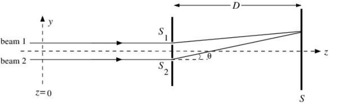Figure 1

III.1 Let the beams 1 and 2 be linearly polarized at $z=0$. The corresponding electric field vectors are given by

\vec{E}_1 = \hat{i}\,E_0 \cos(\omega t) \tag{1a}

\vec{E}_2 = \hat{i}\,E_0 \cos(\omega t) \tag{1b}

where $\hat{i}$ is the unit vector along the $x$-axis, $\omega$ is angular frequency of light and $E_0$ is the amplitude. Find the expression for the intensity of the light $I(\theta )$, that will be observed on the screen where $\theta$ is the angle shown in Fig. (1). Express your answer in terms of $\theta$, $d$, $E_0$, $c$ and $\omega$ where $c$ is the speed of light. Also, note that the intensity is proportional to the time average of the square of the electric field. Here you make take the proportionality constant to be $\beta$. You may ignore the attenuation in the magnitude of the electric fields with distance from the slits to any point on the screen. [1.0 point]

III.2 A perfectly transparent glass slab of thickness $w$ and refractive index $\mu$ is introduced in the path of beam 1 before the slits. Find the expression for the intensity of the light $I(\theta )$ that will be observed on the screen. Express your answer in terms of $\theta$, $d$, $E_0$, $c$, $\omega$, $\mu$ and $w$. [1.0 point]

III.3 An optical device (known as quarter wave plate (QWP)) is introduced in the path of beam 1, before the slits, replacing the glass slab. This device changes the polarization of the beam from the linear polarization state

${\vec{E}}_1=\hat{i}{E}_0\cos (\omega t)$

to a circular polarization state which is given by

\vec{E}_1 = \frac{1}{\sqrt{2}}\left[\hat{i}\,E_0 \cos(\omega t) + \hat{j}\,E_0 \sin(\omega t)\right] \tag{2}

where $\hat{j}$ is the unit vector along the $y$-axis.

Assume that the device does not introduce any additional path difference and that it is perfectly transparent. Note that the tip of the electric field vector traces a circle as time elapses and hence, the beam is said to be circularly polarized. We assume that the angle $\theta$ is small enough so that intensity from slit one does not depend on the angle $\theta$ even for $\hat{j}$ polarization.

III.3.a Find the expression for the intensity $I(\theta )$ of the light that will be observed on the screen. Express your answer in terms of $\theta$, $d$, $E_0$, $c$ and $\omega$.

III.3.b What is the maximum intensity ($I_{max}$)?

III.3.c What is the minimum intensity ($I_{min}$)? [2.0 points]

III.4 Now, consider the experimental setup (see Fig. (2)) in which the beam 1 is subjected to the device (QWP) described in part 3 and,

• a linear polarizer (marked as I), between $z=a$ and $z=b$ which allows only the component of the electric field parallel to an axis ($\hat{i}{}^{\prime }$) to pass through. The unit vector $\hat{i}{}^{\prime }$ is defined as

$\hat{i}{}^{\prime }=\hat{i}\cos \gamma +\hat{j}\sin \gamma$

and,

• another linear polarizer (marked as II) between $z=b$ and $z=c$ which polarizes the beam back to $\hat{i}$ direction.

Thus the beam 1 is back to its original state of polarization. Assume that the polarizers do not introduce any path difference and are perfectly transparent.

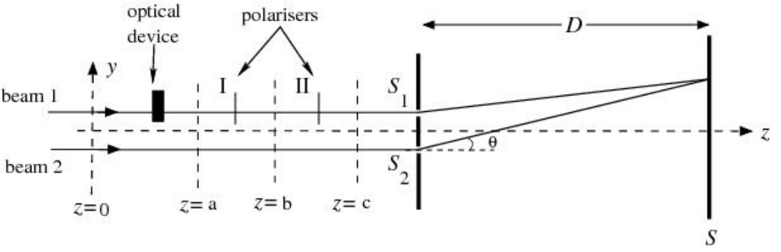Figure 2

III.4.a Write down the expression for the electric field of beam 1 after the first polarizer at $z=b$ $[{\vec{E}}_1(z=b)]$.

III.4.b Write down the expression for the electric field of beam 1 after the second polarizer at $z=c$ $[{\vec{E}}_1(z=c)]$.

III.4.c What is the phase difference ($\alpha$) between the two beams at the slits? [2.0 points]

The most general type of polarization is elliptical polarization. A convenient way of expressing elliptical polarization is to consider it as a superposition of two orthogonal linearly polarized components i.e.

\vec{E} = \hat{i}\,'\,E_0 \cos e \cos(\omega t) + \hat{j}\,'\,E_0 \sin e \sin(\omega t) \tag{3}

where $\hat{i}{}^{\prime }$ and $\hat{j}{}^{\prime }$ and this state of polarization are depicted in Fig. 3.

The tip of the electric field vector traces an ellipse as time elapses. Here $e$ represents the ellipticity and is given by

$\tan e=\frac{\text{Semi-minor axis of the ellipse}}{\text{Semi-major axis of the ellipse}}$

Linear polarization (Eqs. (1)) and circular polarization (Eq. (2)) are special cases of elliptical polarization (Eq. (3)). The two parameters $\gamma (\in [0,\pi ])$ and $e(\in [-\pi /4,\pi /4])$ completely describe the state of polarization.

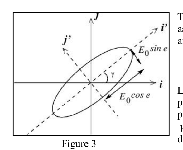Figure 3

The polarization state can also be represented by a point on a sphere of unit radius called the Poincare sphere. The polarization of the beam described in Eq. (3) is represented by a point $P$ on the Poincare sphere (see Fig. 4), then latitude $\angle PCD=2e$ and longitude $\angle ACD=2\gamma$. Here $C$ is the center.

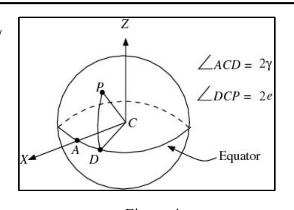Figure 4

III.5 Consider a point on the equator of the Poincare sphere.

III.5.a Write down the electric field (${\vec{E}}_{Eq}$) corresponding to this point.

III.5.b What is its state of polarization? [0.5 point]

III.6 Consider a point at the north pole of the Poincare sphere.

III.6.a Write down the electric field (${\vec{E}}_{NP}$) corresponding to this point.

III.6.b What is its state of polarization? [0.5 point]

III.7 Now, consider the three polarization states of beam 1 as given in part 4. Let the initial polarization (at $z=0$) be represented by a point $A_1$ on the Poincare sphere; after the optical device, let the state (at $z=a$) be represented by point $A_2$ and after the first polarizer (say, at $z=b$), the state be represented by point $A_3$. At $z=c$, the polarization returns to its original state which is represented by $A_1$. Locate these points ($A_1$, $A_2$, and $A_3$) on the Poincare sphere. [1.5 points]

III.8 If these three points ($A_1$, $A_2$, and $A_3$ from the part (III.7)) are joined by great circles on the sphere, a triangle on the surface of the sphere is obtained (Note: A great circle is a circle on the sphere whose center coincides with the center of the sphere). The phase difference $\alpha$ obtained in part 4 and the area $S$ of the curved surface enclosed by the triangle are related to each other. Relate $S$ to $\alpha$. This relationship is general and was obtained by Pancharatnam and the phase difference is called the Pancharatnam phase. [1.5 points]

Fonte: Testo (PDF) — p.1

Topic: Wave Optics, Oscillations & Waves Metodi: Interference & Diffraction Analysis, Superposition Principle, Snell’s Law, Small-Angle Approximation Competenze: Mathematical Modeling, Diagrammatic Reasoning Objects: Slit, Screen

Fase di Pancharatnam

Questo problema riguarda i due fenomeni del fascio associati alla luce, alla sua interferenza, alla polarizzazione e alla sovrapposizione. Il contesto particolare del problema è stato studiato dal fisico indiano S. Pancharatnam (1934-1969).

Considerate la struttura sperimentale mostrata nella figura. (1). Due fasci di luce monocromatiche coerenti (indicati come fasci 1 e 2), che viaggiano nella direzione $z$, si incidono su due fessure strette e sono separate da una distanza $d$ ($S_1{S}_2=d$). Dopo aver attraversato le fessure i due travi si interferiscono e il modello viene osservato sullo schermo $S$. La distanza tra le fessure e lo schermo è $D$ e $D\gg d$. Supponiamo che la larghezza di ciascuna fessura $S_1$ e $S_2$ sia molto inferiore alla lunghezza d’onda della luce.

Figura 1

**III.1 ** Lasciate che i fasci 1 e 2 siano polarizzati linearmente a $z=0$. I vector di campo elettrico corrispondenti sono dati da

\vec{E}_1 = \hat{i}\,E_0 \cos(\omega t) \tag{1a}

\vec{E}_2 = \hat{i}\,E_0 \cos(\omega t) \tag{1b}

se $\hat{i}$ è il vettore unitario lungo l’asse $x$, $\omega$ è la frequenza angolare della luce e $E_0$ è l’ampiezza. Trova l’espressione per l’intensità della luce $I(\theta )$, che verrà osservata sullo schermo dove $\theta$ è l’angolo indicato nella figura. (1). Esprimere la risposta in termini di $\theta$, $d$, $E_0$, $c$ e $\omega$, dove $c$ è la velocità della luce. Si noti inoltre che l’intensità è proporzionale alla media temporale del quadrato del campo elettrico. Qui si fa prendere la costante di proporzionalità a $\beta$. Si può ignorare l’ attenuazione della magnitudine dei campi elettrici con la distanza dalle fessure a qualsiasi punto dello schermo. [1,0 punto]

**III.2 ** In prima delle fessure viene introdotta nella via del fascio 1 una lastra di vetro perfettamente trasparente di spessore $w$ e indice di rifrazione $\mu$. Trova l’espressione per l’intensità della luce $I(\theta )$ che verrà osservata sullo schermo. Esprimi la tua risposta in termini di $\theta$, $d$, $E_0$, $c$, $\omega$, $\mu$ e $w$. [1,0 punto]

III.3 In precedenza delle fessure viene introdotto un dispositivo ottico (noto come piastra a onda di quarto (QWP)) nel percorso del fascio 1, sostituendo la lastra di vetro. Questo dispositivo cambia la polarizzazione del fascio dallo stato di polarizzazione lineare

${\vec{E}}_1=\hat{i}{E}_0\cos (\omega t)$

a uno stato di polarizzazione circolare che è dato da

\vec{E}_1 = \frac{1}{\sqrt{2}}\left[\hat{i}\,E_0 \cos(\omega t) + \hat{j}\,E_0 \sin(\omega t)\right] \tag{2}

dove $\hat{j}$ è il vettore unitario lungo l’asse $y$.

Supponiamo che il dispositivo non introduca alcuna differenza di percorso aggiuntiva e che sia perfettamente trasparente. Si noti che la punta del vettore del campo elettrico traccia un cerchio nel passare del tempo e quindi, il fascio si dice sia polarizzato in modo circolare. Supponiamo che l’angolo $\theta$ sia abbastanza piccolo da non dipendere dall’angolo $\theta$ anche per la polarizzazione $\hat{j}$.

III.3.a Trova l’ espressione per l’ intensità $I(\theta )$ della luce che verrà osservata sullo schermo. Esprimi la tua risposta in termini di $\theta$, $d$, $E_0$, $c$ e $\omega$.

III.3.b Qual è l’ intensità massima ($I_{max}$)?

III.3.c Qual è l’ intensità minima ($I_{min}$)? [2,0 punti]

Ora, considera la configurazione sperimentale (vedi figura 4.2). 2) in cui il fascio 1 è sottoposto al dispositivo (QWP) descritto nella parte 3 e,

• un polarizzatore lineare (indicato come I), tra $z=a$ e $z=b$ che permette di passare solo la componente del campo elettrico parallelo ad un asse ($\hat{i}{}^{\prime }$). Il vettore unitario $\hat{i}{}^{\prime }$ è definito come

$\hat{i}{}^{\prime }=\hat{i}\cos \gamma +\hat{j}\sin \gamma$

e

• un altro polarizzatore lineare (indicato come II) tra $z=b$ e $z=c$ che polarizza il fascio di nuovo nella direzione $\hat{i}$.

Così il raggio 1 è tornato allo stato di polarizzazione originale. Supponiamo che i polarizzatori non introducano alcuna differenza di percorso e siano perfettamente trasparenti.

Figura 2

III.4.a Scrivere l’espressione per il campo elettrico del fascio 1 dopo il primo polarizzatore a $z=b$ $[{\vec{E}}_1(z=b)]$.

III.4.b Scrivere l’espressione per il campo elettrico del fascio 1 dopo il secondo polarizzatore a $z=c$ $[{\vec{E}}_1(z=c)]$.

III.4.c Qual è la differenza di fase ($\alpha$) tra i due fasci delle fessure? [2,0 punti]

Il tipo più generale di polarizzazione è la polarizzazione ellittica. Un modo conveniente per esprimere la polarizzazione ellittica è considerarla come una sovrapposizione di due componenti linearmente polarizzati ortogonali, ovvero:

\vec{E} = \hat{i}\,'\,E_0 \cos e \cos(\omega t) + \hat{j}\,'\,E_0 \sin e \sin(\omega t) \tag{3}

dove $\hat{i}{}^{\prime }$ e $\hat{j}{}^{\prime }$ e questo stato di polarizzazione sono riportati nella figura. 3.

La punta del vettore del campo elettrico traccia un’ellisse nel tempo. Qui $e$ rappresenta l’ellitticità ed è data da

$\tan e=\frac{\text{Semi-minor axis of the ellipse}}{\text{Semi-major axis of the ellipse}}$

Polarizzazione lineare (Eq. 1) e polarizzazione circolare (Eq. 2) sono casi speciali di polarizzazione ellittica (Eq. (3)). I due parametri $\gamma (\in [0,\pi ])$ e $e(\in [-\pi /4,\pi /4])$ descrivono completamente lo stato di polarizzazione.

Figura 3

Lo stato di polarizzazione può anche essere rappresentato da un punto su una sfera di raggio unitario chiamato sfera Poincare. La polarizzazione del raggio descritta in Eq. (3) è rappresentato da un punto $P$ sulla sfera Poincare (cfr. figura 4), poi la latitudine $\angle PCD=2e$ e la longitudine $\angle ACD=2\gamma$. Qui $C$ è il centro.

Figura 4

**III.5 ** Considera un punto sull’equatore della sfera Poincare.

III.5.a Indicare il campo elettrico (${\vec{E}}_{Eq}$) corrispondente a questo punto.

III.5.b Qual è il suo stato di polarizzazione? [0,5 punto]

**III.6 ** Considera un punto al polo nord della sfera Poincare.

III.6.a Indicare il campo elettrico (${\vec{E}}_{NP}$) corrispondente a questo punto.

III.6.b Qual è il suo stato di polarizzazione? [0,5 punto]

Ora, considerate i tre stati di polarizzazione del fascio 1 come indicato nella parte 4. La polarizzazione iniziale (a $z=0$) deve essere rappresentata da un punto $A_1$ sulla sfera Poincare; dopo il dispositivo ottico, lo stato (a $z=a$) deve essere rappresentato da un punto $A_2$ e dopo il primo polarizzatore (per esempio, a $z=b$), lo stato deve essere rappresentato da un punto $A_3$. A $z=c$, la polarizzazione ritorna allo stato originale, rappresentato da $A_1$. Indicare i punti ($A_1$, $A_2$ e $A_3$) sulla sfera Poincare. [1,5 punti]

Se questi tre punti ($A_1$, $A_2$ e $A_3$ della parte (III.7)) sono uniti da grandi cerchi sulla sfera, si ottiene un triangolo sulla superficie della sfera (Nota: Un grande cerchio è un cerchio sulla sfera il cui centro coincide con il centro della sfera). La differenza di fase $\alpha$ ottenuta nella parte 4 e l’area $S$ della superficie curva chiusa dal triangolo sono correlate tra loro. Relazionare $S$ a $\alpha$. Questa relazione è generale e è stata ottenuta da Pancharatnam e la differenza di fase è chiamata fase Pancharatnam. [1,5 punti]

Fonte: Testo (PDF) — p.1

Topic: Wave Optics, Oscillations & Waves Metodi: Interference & Diffraction Analysis, Superposition Principle, Snell’s Law, Small-Angle Approximation Competenze: Mathematical Modeling, Diagrammatic Reasoning Objects: Slit, Screen