APhO 2013 — Teorica

Conductors in Conducting Liquid

A system consisting of two conductor bodies is immersed in a uniform dielectric and weakly conducting liquid. When a constant voltage difference is applied between both conductors, the system has both electric and magnetic fields. In this problem we will investigate this system.

1. (0.4 pts) First consider an infinitely long line with charge per unit length $\lambda$ in vacuum. Calculate the electric field $\mathbf{E}(r)$ due to the line.

2. (0.4 pts) The potential due to the line charge could be written as $V(r)=f(r)+K,$ where $K$ is a constant. Determine $f(r)$.

3. (0.7 pts) Calculate the potential in all space $V(x,y,z)$ due to an infinitely long line with charge per unit length $\lambda$ at $x=-b,y=0$ and another infinitely long line with charge per unit length $-\lambda$ at $x=b,y=0$. Both lines are parallel to the $z$-axis. Take $V=0$ at the origin. Sketch the equipotential surfaces.

For the following questions, ignore any edge effects.

4. (2.0 pts) Now consider two identical conducting cylinders, both with radius $R=3a$ in vacuum. The length of each cylinder is the same and much larger than its radius ($l\gg R$). The axes of both cylinders are on the $xz$-plane and parallel to the $z$-axis, one at $x=-5a,y=0$ and the other at $x=5a,y=0$. An electrical potential difference of $V_0$ is applied between the two cylinders (the cylinder at $x=-5a$ has the higher potential) by connecting them to a battery. Calculate the potential in all regions. Take $V=0$ at the origin.

5. (0.5 pts) Calculate the capacitance $C$ of the system.

6. (1.0 pts) Now both cylinders are totally immersed in a weakly conducting liquid with conductivity $\sigma$. Calculate the total current that flows between both cylinders. Assume the permittivity of the liquid is equal to that of vacuum, $ϵ={ϵ}_0$.

7. (0.5 pts) Calculate the resistance $R$ of the system. Calculate $RC$ of the system.

8. (1.5 pts) Calculate the magnetic field due to the current in question 6. Assume that the permeability of the liquid is equal to that of vacuum, $\mu ={\mu }_0$.

Notes $\int \frac{dx}{x^2+a^2}=\arctan \frac{x}{a}+\text{const}$

Fonte: Testo (PDF) — p.1

Topic: Electrostatics, Electromagnetism Metodi: Gauss’s Law, Electric Potential Method, Superposition Principle, Ampère’s Law Competenze: Mathematical Modeling, Physical Reasoning Objects: Cylinder, Battery

Conduttori nel conduttore di liquidi

Un sistema composto da due corpi conduttori è immerso in un liquido dielettrico uniforme e debole conduttore. Quando si applica una differenza di tensione costante tra entrambi i conduttori, il sistema ha campi elettrici e magnetici. In questo problema, esamineremo questo sistema.

1. **(0,4 pts) ** Primo consideriamo una linea infinitamente lunga con carica per unità di lunghezza $\lambda$ nel vuoto. Calcolare il campo elettrico $\mathbf{E}(r)$ dovuto alla linea.

2. **(0,4 pts) ** Il potenziale dovuto alla carica della linea potrebbe essere scritto come $V(r)=f(r)+K,$ in cui $K$ è una costante. Determina $f(r)$.

3. **(0,7 pts) ** Calcolare il potenziale in tutto lo spazio $V(x,y,z)$ dovuto a una linea infinitamente lunga con carica per lunghezza unità $\lambda$ a $x=-b,y=0$ e ad un’altra linea infinitamente lunga con carica per lunghezza unità $-\lambda$ a $x=b,y=0$. Entrambe le linee sono parallele all’asse $z$. Prendi $V=0$ all’origine. Segna le superfici equipotenziali.

Per le seguenti domande, ignora gli effetti negativi.

4. **(2,0 pts) ** Ora consideriamo due cilindri conduttori identici, entrambi con raggio $R=3a$ nel vuoto. La lunghezza di ciascun cilindro è uguale e molto maggiore del suo raggio ($l\gg R$). Gli assi di entrambi i cilindri sono situati sul piano $xz$ e paralleli all’asse $z$, uno a $x=-5a,y=0$ e l’altro a $x=5a,y=0$. Si applica una differenza di potenziale elettrico di $V_0$ tra i due cilindri (il cilindro a $x=-5a$ ha il potenziale più elevato) collegandoli a una batteria. Calcolare il potenziale in tutte le regioni. Prendi $V=0$ all’origine.

5. **(0,5 pts) ** Calcolare la capacità $C$ del sistema.

6. Ora entrambi i cilindri sono completamente immersi in un liquido debole con conductività $\sigma$. Calcolare la corrente totale che scorre tra i due cilindri. Supponiamo che la permissività del liquido sia uguale a quella del vuoto, $ϵ={ϵ}_0$.

7. **(0,5 pts) ** Calcolare la resistenza $R$ del sistema. Calcolare $RC$ del sistema.

8. **(1,5 pts) ** Calcolare il campo magnetico dovuto alla corrente in questione 6. Supponiamo che la permeabilità del liquido sia uguale a quella del vuoto, $\mu ={\mu }_0$.

Noti $\int \frac{dx}{x^2+a^2}=\arctan \frac{x}{a}+\text{const}$

Fonte: Testo (PDF) — p.1

Topic: Electrostatics, Electromagnetism Metodi: Gauss’s Law, Electric Potential Method, Superposition Principle, Ampère’s Law Competenze: Mathematical Modeling, Physical Reasoning Objects: Cylinder, Battery

Relativistic Correction on GPS Satellite

Global Positioning System (GPS) is a navigation technology which uses signal from satellites to determine the position of an object (for example an airplane). However, due to the satellites’ high speed movement in orbit, there should be a special relativistic correction, and due to their high altitude, there should be a general relativistic correction. Both corrections seem to be small but are very important for precise measurement of position. We will explore both corrections in this problem.

First we will investigate the special relativistic effect on an accelerated particle. We consider two types of frame, the first one is the rest frame (called $S$ or Earth’s frame), where the particle is at rest initially. The other is the proper frame (called $S^{\prime }$), a frame that instantaneously moves together with the accelerated particle. Note that this is not an accelerated frame, it is a constant velocity frame that at a particular moment has the same velocity with the accelerated particle. At that short moment, the time rate experienced by the particle is the same as the proper frame’s time rate. Of course this proper frame is only good for an infinitesimally short time, and then we need to define a new proper frame afterward. At the beginning we synchronize the particle’s clock with the clock in the rest frame by setting them to zero, $t=\tau =0$ ($t$ is the time in the rest frame, and $\tau$ is the time shown by the particle’s clock).

By applying the equivalence principle, we can obtain general relativistic effects from special relativistic results which does not involve complicated metric tensor calculations. By combining the special and general relativistic effects, we can calculate the corrections needed for a GPS (global positioning system) satellite to provide accurate positioning.

Some mathematics formulas that might be useful

• $\sinh x=\frac{e^x-e^{-x}}{2}$
• $\cosh x=\frac{e^x+e^{-x}}{2}$
• $\tanh x=\frac{\sinh x}{\cosh x}$
• $1+{\sinh }^{2}x={\cosh }^{2}x$
• $\sinh (x-y)=\sinh x\cosh y-\cosh x\sinh y$
• $\int \frac{dx}{(1-x^2{)}^{3/2}}=\frac{x}{\sqrt{1-x^2}}+C$
• $\int \frac{dx}{1-x^2}=\ln \sqrt{\frac{1+x}{1-x}}+C$

Part A. Single Accelerated Particle (2.8 points)

Consider a particle with a rest mass $m$ under a constant and uniform force field $F$ (defined in the rest frame) pointing in the positive $x$ direction. Initially ($t=\tau =0$) the particle is at rest at the origin ($x=0$).

1. (0.5 pts) When the velocity of the particle is $v$, calculate the acceleration of the particle, $a$ (with respect to the rest frame).

2. (0.5 pts) Calculate the velocity of the particle $\beta (t)=\frac{v(t)}{c}$ at time $t$ (in rest frame), in terms of $F$, $m$, $t$ and $c$.

3. (0.3 pts) Calculate the position of the particle $x(t)$ at time $t$, in terms of $F$, $m$, $t$ and $c$.

4. (0.7 pts) Show that the proper acceleration of the particle, $a_0\equiv g=F/m$, is a constant. The proper acceleration is the acceleration of the particle measured in the instantaneous proper frame.

5. (0.4 pts) Calculate the velocity of the particle $\beta (\tau )$, when the time as experienced by the particle is $\tau$. Express the answer in $g$, $\tau$, and $c$.

6. (0.4 pts) Also calculate the time $t$ in the rest frame in terms of $g$, $\tau$, and $c$.

Part B. Flight Time (2.0 points)

The first part has not taken into account the flight time of the information to arrive to the observer. This part is the only part in the whole problem where the flight time is considered. The particle moves as in part A.

1. (1.2 pts) At a certain moment, the time experienced by the particle is $\tau$. What reading $t_0$ on a stationary clock located at $x=0$ will be observed by the particle? After a long period of time, does the observed reading $t_0$ approach a certain value? If so, what is the value?

2. (0.8 pts) Now consider the opposite point of view. If an observer at the initial point ($x=0$) is observing the particle’s clock when the observer’s time is $t$, what is the reading of the particle’s clock ${\tau }_0$? After a long period of time, will this reading approach a certain value? If so, what is the value?

Part C. Minkowski Diagram (1.0 points)

In many occasions, it is very useful to illustrate relativistic events using a diagram, called as Minkowski Diagram. To make the diagram, we just need to use Lorentz transformation between the rest frame $S$ and the moving frame $S^{\prime }$ that move with velocity $v=\beta c$ with respect to the rest frame.

$x=\gamma (x^{\prime }+\beta c{t}^{\prime }),$ $ct=\gamma (c{t}^{\prime }+\beta x^{\prime }),$ $x^{\prime }=\gamma (x-\beta ct),$ $c{t}^{\prime }=\gamma (ct-\beta x).$ $\gamma =\frac{1}{\sqrt{1-\frac{v^2}{c^2}}}$

Let’s choose $x$ and $ct$ as the orthogonal axes. A point $(x^{\prime },c{t}^{\prime })=(1,0)$ in the moving frame $S^{\prime }$ has a coordinate $(x,ct)=(\gamma ,\gamma \beta )$ in the rest frame $S$. The line connecting this point and the origin defines the $x^{\prime }$ axis. Another point $(x^{\prime },c{t}^{\prime })=(0,1)$ in the moving frame $S^{\prime }$ has a coordinate $(x,ct)=(\gamma \beta ,\gamma )$ in the rest frame $S$. The line connecting this point and the origin defines the $c{t}^{\prime }$ axis. The angle between the $x$ and $x^{\prime }$ axis is $\theta$, where $\tan \theta =\beta$. A unit length in the moving frame $S^{\prime }$ is equal to $\gamma \sqrt{1+{\beta }^2}=\sqrt{\frac{1+{\beta }^2}{1-{\beta }^2}}$ in the rest frame $S$.

To get a better understanding of Minkowski diagram, let us take a look at this example. Consider a stick of proper length $L$ in a moving frame $S^{\prime }$. We would like to find the length of the stick in the rest frame $S$. Consider the figure below.

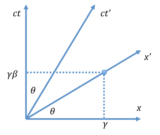
The stick is represented by the segment $AC$. The length $AC$ is equal to $\sqrt{\frac{1+{\beta }^2}{1-{\beta }^2}}L$ in the $S$ frame. The stick length in the $S$ frame is represented by the line $AB$.

$$\begin{array}{rl}AB& =AD-BD\\ & =AC\cos \theta -AC\sin \theta \tan \theta \\ & =L\sqrt{1-{\beta }^2}\end{array}$$

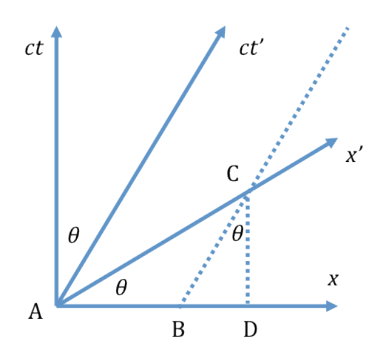
1. (0.5 pts) Using a Minkowski diagram, calculate the length of a stick with proper length $L$ in the rest frame, as measured in the moving frame.

2. (0.5 pts) Now consider the case in part A. Plot the time $ct$ versus the position $x$ of the particle. Draw the $x^{\prime }$ axis and $c{t}^{\prime }$ axis when $\frac{v}{c}=1$ in the same graph using length scale $x(c^2/g)$ and $ct(c^2/g)$.

Part D. Two Accelerated Particles (2.3 points)

For this part, we will consider two accelerated particles, both of them have the same proper acceleration $g$ in the positive $x$ direction, but the first particle starts from $x=0$, while the second particle starts from $x=L$. Remember, DO NOT consider the flight time in this part.

1. (0.3 pts) After a while, an observer in the rest frame makes an observation. The first particle’s clock shows time at ${\tau }_1$. What is the reading of the second clock ${\tau }_2$, according to the observer in the rest frame.

2. (1.0 pts) Now consider the observation from the first particle’s frame. At a certain moment, an observer that moves together with the first particle observed that the reading of his own clock is ${\tau }_1$. At the same time, he observed the second particle’s clock, and the reading is ${\tau }_2$. Show that $\sinh \frac{g}{c}({\tau }_1-{\tau }_2)=C_1\sinh \frac{g{\tau }_1}{c},$ where $C_1$ is a constant. Determine $C_1$.

3. (1.0 pts) The first particle will see the second particle move away from him. Show that the rate of change of the distance between the two particles according to the first particle is $\frac{d{L}^{\prime }}{d{\tau }_1}=C_2\frac{\sinh \frac{g{\tau }_1}{c}}{\cosh \frac{g}{c}({\tau }_1-{\tau }_2)},$ where $C_2$ is a constant. Determine $C_2$.

Part E. Uniformly Accelerated Frame (2.7 points)

In this part we will arrange the proper acceleration of the particles, so that the distance between both particles are constant according to each particle. Initially both particles are at rest, the first particle is at $x=0$, while the second particle is at $x=L$.

1. (0.8 pts) The first particle has a proper acceleration $g_1$ in the positive $x$ direction. When it is being accelerated, there exists a fixed point in the rest frame at $x=x_p$ that has a constant distance from the first particle, according to the first particle throughout the motion. Determine $x_p$.

2. (1.3 pts) Given the proper acceleration of the first particle is $g_1$, determine the proper acceleration of the second particle $g_2$, so that the distance between the two particles are constant according to the first particle.

3. (0.6 pts) What is the ratio of time rate of the second particle to the first particle $\frac{d{\tau }_2}{d{\tau }_1}$, according to the first particle.

Part F. Correction for GPS (2.2 points)

Part E indicates that the time rate of clocks at different altitude will not be the same, even though there is no relative movement between those clocks. According to the equivalence principle in general relativity, an observer in a small closed room could not tell the difference between a gravity pull $g$ and the fictitious force from accelerated frame with acceleration $g$. So we can conclude that two clocks at different gravitational potential will have different rate.

Now let consider a GPS satellite that orbiting the Earth with a period of 12 hours.

1. (0.6 pts) If the gravitational acceleration on the Earth’s surface is $9.78\mathrm{m}{\mathrm{s}}^{-2}$, and the Earth’s radius is $6380\mathrm{km}$, what is the radius of the GPS satellite orbit? What is the velocity of the satellite? Calculate the numerical values of the radius and the velocity.

2. (1.2 pts) After one day, the clock reading on the Earth surface and the satellite will differ due to both special and general relativistic effects. Calculate the difference due to each effect for one day. Calculate the total difference for one day. Which clock is faster, a clock on the Earth’s surface or the satellite’s clock?

3. (0.4 pts) After one day, estimate the error in position due to this effect?

Fonte: Testo (PDF) — p.1

Topic: Special Relativity, Gravitation Metodi: Lorentz Transformation, Differential Equations, Calculus-Integration, Kepler’s Laws Competenze: Mathematical Modeling, Diagrammatic Reasoning Objects: Satellite, Planet

Correzione relativistica sul satellite GPS

Il Sistema di Posizionamento Globale (GPS) è una tecnologia di navigazione che usa segnali dai satelliti per determinare la posizione di un oggetto (per esempio un aereo). Tuttavia, a causa del moto ad alta velocità dei satelliti in orbita, dovrebbe esserci una correzione relativistica ristretta, e a causa della loro elevata altitudine, dovrebbe esserci una correzione relativistica generale. Entrambe le correzioni sembrano piccole ma sono molto importanti per una misura precisa della posizione. Esploreremo entrambe le correzioni in questo problema.

Per prima cosa studieremo l’effetto relativistico ristretto su una particella accelerata. Consideriamo due tipi di sistema di riferimento: il primo è il sistema di quiete (chiamato $S$ o sistema della Terra), dove la particella è inizialmente a riposo. L’altro è il sistema proprio (chiamato $S^{\prime }$), un sistema che si muove istantaneamente insieme alla particella accelerata. Nota che questo non è un sistema accelerato, è un sistema a velocità costante che in un particolare istante ha la stessa velocità della particella accelerata. In quel breve istante, il ritmo del tempo sperimentato dalla particella è lo stesso del ritmo del tempo del sistema proprio. Naturalmente questo sistema proprio è valido solo per un tempo infinitesimamente breve, e poi dobbiamo definire un nuovo sistema proprio in seguito. All’inizio sincronizziamo l’orologio della particella con l’orologio nel sistema di quiete azzerandoli, $t=\tau =0$ ($t$ è il tempo nel sistema di quiete, e $\tau$ è il tempo indicato dall’orologio della particella).

Applicando il principio di equivalenza, possiamo ottenere gli effetti relativistici generali dai risultati relativistici ristretti, il che non comporta complicati calcoli con il tensore metrico. Combinando gli effetti relativistici ristretti e generali, possiamo calcolare le correzioni necessarie a un satellite GPS (sistema di posizionamento globale) per fornire un posizionamento accurato.

Alcune formule matematiche che potrebbero essere utili

• $\sinh x=\frac{e^x-e^{-x}}{2}$
• $\cosh x=\frac{e^x+e^{-x}}{2}$
• $\tanh x=\frac{\sinh x}{\cosh x}$
• $1+{\sinh }^{2}x={\cosh }^{2}x$
• $\sinh (x-y)=\sinh x\cosh y-\cosh x\sinh y$
• $\int \frac{dx}{(1-x^2{)}^{3/2}}=\frac{x}{\sqrt{1-x^2}}+C$
• $\int \frac{dx}{1-x^2}=\ln \sqrt{\frac{1+x}{1-x}}+C$

Parte A. Singola particella accelerata (2.8 punti)

Considera una particella con massa a riposo $m$ sotto un campo di forza costante e uniforme $F$ (definito nel sistema di quiete) diretto nella direzione $x$ positiva. Inizialmente ($t=\tau =0$) la particella è a riposo nell’origine ($x=0$).

1. (0.5 pts) Quando la velocità della particella è $v$, calcola l’accelerazione della particella, $a$ (rispetto al sistema di quiete).

2. (0.5 pts) Calcola la velocità della particella $\beta (t)=\frac{v(t)}{c}$ al tempo $t$ (nel sistema di quiete), in termini di $F$, $m$, $t$ e $c$.

3. (0.3 pts) Calcola la posizione della particella $x(t)$ al tempo $t$, in termini di $F$, $m$, $t$ e $c$.

4. (0.7 pts) Mostra che l’accelerazione propria della particella, $a_0\equiv g=F/m$, è una costante. L’accelerazione propria è l’accelerazione della particella misurata nel sistema proprio istantaneo.

5. (0.4 pts) Calcola la velocità della particella $\beta (\tau )$, quando il tempo sperimentato dalla particella è $\tau$. Esprimi la risposta in $g$, $\tau$ e $c$.

6. (0.4 pts) Calcola inoltre il tempo $t$ nel sistema di quiete in termini di $g$, $\tau$ e $c$.

Parte B. Tempo di volo (2.0 punti)

La prima parte non ha tenuto conto del tempo di volo dell’informazione per arrivare all’osservatore. Questa parte è l’unica parte in tutto il problema in cui si considera il tempo di volo. La particella si muove come nella parte A.

1. (1.2 pts) In un certo istante, il tempo sperimentato dalla particella è $\tau$. Quale lettura $t_0$ su un orologio stazionario posto in $x=0$ sarà osservata dalla particella? Dopo un lungo periodo di tempo, la lettura osservata $t_0$ tende a un certo valore? Se sì, qual è il valore?

2. (0.8 pts) Considera ora il punto di vista opposto. Se un osservatore nel punto iniziale ($x=0$) sta osservando l’orologio della particella quando il tempo dell’osservatore è $t$, qual è la lettura dell’orologio della particella ${\tau }_0$? Dopo un lungo periodo di tempo, questa lettura tenderà a un certo valore? Se sì, qual è il valore?

Parte C. Diagramma di Minkowski (1.0 punti)

In molte occasioni, è molto utile illustrare gli eventi relativistici usando un diagramma, chiamato diagramma di Minkowski. Per costruire il diagramma, basta usare la trasformazione di Lorentz tra il sistema di quiete $S$ e il sistema in moto $S^{\prime }$ che si muove con velocità $v=\beta c$ rispetto al sistema di quiete.

$x=\gamma (x^{\prime }+\beta c{t}^{\prime }),$ $ct=\gamma (c{t}^{\prime }+\beta x^{\prime }),$ $x^{\prime }=\gamma (x-\beta ct),$ $c{t}^{\prime }=\gamma (ct-\beta x).$ $\gamma =\frac{1}{\sqrt{1-\frac{v^2}{c^2}}}$

Scegliamo $x$ e $ct$ come assi ortogonali. Un punto $(x^{\prime },c{t}^{\prime })=(1,0)$ nel sistema in moto $S^{\prime }$ ha coordinata $(x,ct)=(\gamma ,\gamma \beta )$ nel sistema di quiete $S$. La retta che congiunge questo punto e l’origine definisce l’asse $x^{\prime }$. Un altro punto $(x^{\prime },c{t}^{\prime })=(0,1)$ nel sistema in moto $S^{\prime }$ ha coordinata $(x,ct)=(\gamma \beta ,\gamma )$ nel sistema di quiete $S$. La retta che congiunge questo punto e l’origine definisce l’asse $c{t}^{\prime }$. L’angolo tra l’asse $x$ e l’asse $x^{\prime }$ è $\theta$, dove $\tan \theta =\beta$. Un’unità di lunghezza nel sistema in moto $S^{\prime }$ è uguale a $\gamma \sqrt{1+{\beta }^2}=\sqrt{\frac{1+{\beta }^2}{1-{\beta }^2}}$ nel sistema di quiete $S$.

Per capire meglio il diagramma di Minkowski, guardiamo questo esempio. Considera un’asta di lunghezza propria $L$ in un sistema in moto $S^{\prime }$. Vogliamo trovare la lunghezza dell’asta nel sistema di quiete $S$. Considera la figura seguente.

L’asta è rappresentata dal segmento $AC$. La lunghezza $AC$ è uguale a $\sqrt{\frac{1+{\beta }^2}{1-{\beta }^2}}L$ nel sistema $S$. La lunghezza dell’asta nel sistema $S$ è rappresentata dal segmento $AB$.

$$\begin{array}{rl}AB& =AD-BD\\ & =AC\cos \theta -AC\sin \theta \tan \theta \\ & =L\sqrt{1-{\beta }^2}\end{array}$$

1. (0.5 pts) Usando un diagramma di Minkowski, calcola la lunghezza di un’asta di lunghezza propria $L$ nel sistema di quiete, come misurata nel sistema in moto.

2. (0.5 pts) Considera ora il caso della parte A. Traccia il tempo $ct$ in funzione della posizione $x$ della particella. Disegna l’asse $x^{\prime }$ e l’asse $c{t}^{\prime }$ quando $\frac{v}{c}=1$ nello stesso grafico usando la scala di lunghezza $x(c^2/g)$ e $ct(c^2/g)$.

Parte D. Due particelle accelerate (2.3 punti)

Per questa parte, considereremo due particelle accelerate, entrambe con la stessa accelerazione propria $g$ nella direzione $x$ positiva, ma la prima particella parte da $x=0$, mentre la seconda particella parte da $x=L$. Ricorda, NON considerare il tempo di volo in questa parte.

1. (0.3 pts) Dopo un po’, un osservatore nel sistema di quiete effettua un’osservazione. L’orologio della prima particella indica il tempo ${\tau }_1$. Qual è la lettura del secondo orologio ${\tau }_2$, secondo l’osservatore nel sistema di quiete.

2. (1.0 pts) Considera ora l’osservazione dal sistema della prima particella. In un certo istante, un osservatore che si muove insieme alla prima particella osserva che la lettura del proprio orologio è ${\tau }_1$. Nello stesso istante, osserva l’orologio della seconda particella, e la lettura è ${\tau }_2$. Mostra che $\sinh \frac{g}{c}({\tau }_1-{\tau }_2)=C_1\sinh \frac{g{\tau }_1}{c},$ dove $C_1$ è una costante. Determina $C_1$.

3. (1.0 pts) La prima particella vedrà la seconda particella allontanarsi da essa. Mostra che il tasso di variazione della distanza tra le due particelle secondo la prima particella è $\frac{d{L}^{\prime }}{d{\tau }_1}=C_2\frac{\sinh \frac{g{\tau }_1}{c}}{\cosh \frac{g}{c}({\tau }_1-{\tau }_2)},$ dove $C_2$ è una costante. Determina $C_2$.

Parte E. Sistema uniformemente accelerato (2.7 punti)

In questa parte disporremo l’accelerazione propria delle particelle in modo che la distanza tra le due particelle sia costante secondo ciascuna particella. Inizialmente entrambe le particelle sono a riposo, la prima particella è in $x=0$, mentre la seconda particella è in $x=L$.

1. (0.8 pts) La prima particella ha accelerazione propria $g_1$ nella direzione $x$ positiva. Mentre viene accelerata, esiste un punto fisso nel sistema di quiete in $x=x_p$ che ha una distanza costante dalla prima particella, secondo la prima particella durante tutto il moto. Determina $x_p$.

2. (1.3 pts) Data l’accelerazione propria della prima particella $g_1$, determina l’accelerazione propria della seconda particella $g_2$, così che la distanza tra le due particelle sia costante secondo la prima particella.

3. (0.6 pts) Qual è il rapporto tra il ritmo del tempo della seconda particella e quello della prima particella $\frac{d{\tau }_2}{d{\tau }_1}$, secondo la prima particella.

Parte F. Correzione per il GPS (2.2 punti)

La Parte E indica che il ritmo del tempo di orologi a diversa altitudine non sarà lo stesso, anche se non c’è moto relativo tra tali orologi. Secondo il principio di equivalenza in relatività generale, un osservatore in una piccola stanza chiusa non potrebbe distinguere tra un’attrazione gravitazionale $g$ e la forza fittizia da un sistema accelerato con accelerazione $g$. Quindi possiamo concludere che due orologi a diverso potenziale gravitazionale avranno ritmi diversi.

Consideriamo ora un satellite GPS che orbita attorno alla Terra con un periodo di 12 ore.

1. (0.6 pts) Se l’accelerazione gravitazionale alla superficie della Terra è $9.78\mathrm{m}{\mathrm{s}}^{-2}$, e il raggio della Terra è $6380\mathrm{km}$, qual è il raggio dell’orbita del satellite GPS? Qual è la velocità del satellite? Calcola i valori numerici del raggio e della velocità.

2. (1.2 pts) Dopo un giorno, la lettura dell’orologio sulla superficie della Terra e quella del satellite differiranno a causa di entrambi gli effetti relativistici, ristretto e generale. Calcola la differenza dovuta a ciascun effetto per un giorno. Calcola la differenza totale per un giorno. Quale orologio è più veloce, un orologio sulla superficie della Terra o l’orologio del satellite?

3. (0.4 pts) Dopo un giorno, stima l’errore di posizione dovuto a questo effetto?

Fonte: Testo (PDF) — p.1

Topic: Special Relativity, Gravitation Metodi: Lorentz Transformation, Differential Equations, Calculus-Integration, Kepler’s Laws Competenze: Mathematical Modeling, Diagrammatic Reasoning Objects: Satellite, Planet

Physics of Spin

All matter in the universe has fundamental properties called spin, besides their mass and charge. Spin is an intrinsic form of angular momentum carried by particles. Despite the fact that quantum mechanics is needed for a full treatment of spin, we can still study the physics of spin using the usual classical formalism. In this problem, we are investigating the influence of magnetic field on spin using its classical analogue.

The classical torque equation of spin is given by $\mathbf{\tau }=\frac{d\mathbf{L}}{dt}=\mathbf{\mu }\times \mathbf{B}.$ In this case, the angular momentum $\mathbf{L}$ represents the “intrinsic” spin of the particles, $\mathbf{\mu }$ is the magnetic moment of the particles, and $\mathbf{B}$ is magnetic field. The spin of a particle is associated with a magnetic moment via the equation $\mathbf{\mu }=-\gamma \mathbf{L}$ where $\gamma$ is the gyromagnetic ratio.

In this problem, the term “frequency” means angular frequency (rad/s), which is a scalar quantity. All bold letters represent vectors; otherwise they represent scalars.

Part A. Larmor precession (1.6 points)

1. (0.8 pts) Prove that the magnitude of magnetic moment $\mu$ is always constant under the influence of a magnetic field $\mathbf{B}$. For a special case of stationary (constant) magnetic field, also show that the angle between $\mathbf{\mu }$ and $\mathbf{B}$ is constant. (Hint: You can use properties of vector products.)

2. (0.8 pts) A uniform magnetic field $\mathbf{B}$ exists and it makes an angle $\varphi$ with a particle’s magnetic moment $\mathbf{\mu }$. Due to the torque by the magnetic field, the magnetic moment $\mathbf{\mu }$ rotates around the field $\mathbf{B}$, which is also known as Larmor precession. Determine the Larmor precession frequency ${\omega }_0$ of the magnetic moment with respect to $\mathbf{B}=B_0\mathbf{k}$.

Part B. Rotating frame (3.4 points)

In this section, we choose a rotating frame $S^{\prime }$ as our frame of reference. The rotating frame $S^{\prime }=(x^{\prime },y^{\prime },z^{\prime })$ rotates with an angular velocity $\omega \mathbf{k}$ as seen by an observer in the laboratory frame $S=(x,y,z)$, where the axes $x^{\prime },y^{\prime },z^{\prime }$ intersect with $x,y,z$ at time $t=0$. Any vector $\mathbf{A}=A_x\mathbf{i}+A_y\mathbf{j}+A_z\mathbf{k}$ in a lab frame can be written as $\mathbf{A}=A_{x^{\prime }}{\mathbf{i}}^{\prime }+A_{y^{\prime }}{\mathbf{j}}^{\prime }+A_{z^{\prime }}{\mathbf{k}}^{\prime }$ in the rotating frame $S^{\prime }$. The time derivative of the vector becomes $\frac{d\mathbf{A}}{dt}=\frac{d{A}_{x^{\prime }}}{dt}{\mathbf{i}}^{\prime }+\frac{d{A}_{y^{\prime }}}{dt}{\mathbf{j}}^{\prime }+\frac{d{A}_{z^{\prime }}}{dt}{\mathbf{k}}^{\prime }+A_{x^{\prime }}\frac{d{\mathbf{i}}^{\prime }}{dt}+A_{y^{\prime }}\frac{d{\mathbf{j}}^{\prime }}{dt}+A_{z^{\prime }}\frac{d{\mathbf{k}}^{\prime }}{dt}$ ${\left(\frac{d\mathbf{A}}{dt}\right)}_{\mathrm{lab}}={\left(\frac{d\mathbf{A}}{dt}\right)}_{\mathrm{rot}}+\omega \mathbf{k}\times \mathbf{A},$ where ${\left(\frac{d\mathbf{A}}{dt}\right)}_{\mathrm{lab}}$ is the time derivative of vector $\mathbf{A}$ seen by an observer in the lab frame, and ${\left(\frac{d\mathbf{A}}{dt}\right)}_{\mathrm{rot}}$ is the time derivative seen by an observer in the rotating frame. For all the following problems in this part, the answers are referred to the rotating frame $S^{\prime }$.

1. (0.8 pts) Show that the time evolution of the magnetic moment follows the equation ${\left(\frac{d\mathbf{\mu }}{dt}\right)}_{\mathrm{rot}}=-\gamma \mathbf{\mu }\times {\mathbf{B}}_{\mathrm{eff}},$ where ${\mathbf{B}}_{\mathrm{eff}}=\mathbf{B}-\frac{\omega }{\gamma }{\mathbf{k}}^{\prime }$ is the effective magnetic field.

2. (0.4 pts) For $\mathbf{B}=B_0\mathbf{k}$, what is the new precession frequency $\Delta$ in terms of ${\omega }_0$ and $\omega$?

3. (1.2 pts) Now, let us consider the case of a time-varying magnetic field. Besides a constant magnetic field, we also apply a rotating magnetic field $\mathbf{b}(t)=b(\cos \omega t\mathbf{i}+\sin \omega t\mathbf{j})$, so $\mathbf{B}=B_0\mathbf{k}+\mathbf{b}(t)$. Show that the new Larmor precession frequency of the magnetic moment is $\Omega =\gamma \sqrt{{\left(B_0-\frac{\omega }{\gamma }\right)}^2+b^2}.$

4. (1.0 pts) Instead of applying the field $\mathbf{b}(t)=b(\cos \omega t\mathbf{i}+\sin \omega t\mathbf{j})$, now we apply $\mathbf{b}(t)=b(\cos \omega t\mathbf{i}-\sin \omega t\mathbf{j})$, which rotates in the opposite direction and hence $\mathbf{B}=B_0\mathbf{k}+b(\cos \omega t\mathbf{i}-\sin \omega t\mathbf{j})$. What is the effective magnetic field ${\mathbf{B}}_{\mathrm{eff}}$ for this case (in terms of the unit vectors ${\mathbf{i}}^{\prime },{\mathbf{j}}^{\prime },{\mathbf{k}}^{\prime }$)? What is its time average, $\overline{{\mathbf{B}}_{\mathrm{eff}}}$ (recall that $\overline{\cos 2\pi t/T}=\overline{\sin 2\pi t/T}=0$)?

Part C. Rabi oscillation (3.0 points)

For an ensemble of $N$ particles under the influence of a large magnetic field, the spin can have two quantum states: “up” and “down”. Consequently, the total population of spin up $N_{\uparrow }$ and down $N_{\downarrow }$ obeys the equation $N_{\uparrow }+N_{\downarrow }=N.$ The difference of spin up population and spin down population yields the macroscopic magnetization along the $z$ axis: $M=(N_{\uparrow }-N_{\downarrow })\mu =N{\mu }_z.$ In a real experiment, two magnetic fields are usually applied, a large bias field $B_0\mathbf{k}$ and an oscillating field with amplitude $2b$ perpendicular to the bias field ($b\ll B_0$). Initially, only the large bias is applied, causing all the particles lie in the spin up states ($\mathbf{\mu }$ is oriented in the $z$-direction at $t=0$). Then, the oscillating field is turned on, where its frequency $\omega$ is chosen to be in resonance with the Larmor precession frequency ${\omega }_0$, i.e. $\omega ={\omega }_0$. In other words, the total field after time $t=0$ is given by $\mathbf{B}(t)=B_0\mathbf{k}+2b\cos {\omega }_{0}t\mathbf{i}.$

1. (1.2 pts) In the rotating frame $S^{\prime }$, show that the effective field can be approximated by ${\mathbf{B}}_{\mathrm{eff}}\approx b{\mathbf{i}}^{\prime },$ which is commonly known as rotating wave approximation. What is the precession frequency $\Omega$ in frame $S^{\prime }$?

2. (0.6 pts) Determine the angle $\alpha$ that $\mathbf{\mu }$ makes with ${\mathbf{B}}_{\mathrm{eff}}$. Also, prove that the magnetization varies with time as $M(t)=N\mu \cos \Omega t.$

3. (1.2 pts) Under the application of magnetic field described above, determine the fractional population of each spin up $P_{\uparrow }=N_{\uparrow }/N$ and spin down $P_{\downarrow }=N_{\downarrow }/N$ as a function of time. Plot $P_{\uparrow }(t)$ and $P_{\downarrow }(t)$ on the same graph vs. time $t$. The alternating spin up and spin down population as a function of time is called Rabi oscillation.

Part D. Measurement incompatibility (2.0 points)

Spin is in fact a vector quantity; but due to its quantum properties, we cannot measure each of its components simultaneously (i.e. we can know both $|\mathbf{\mu }|$ and ${\mu }_z$ as in above problems; but not all $|\mathbf{\mu }|,{\mu }_x,{\mu }_y,$ and ${\mu }_z$ simultaneously). In this problem, we will do a calculation based on the Heisenberg uncertainty principle (using the relation $\Delta p_q\Delta q\ge \hslash$) to show how these measurements are incompatible with each other.

1. (1.0 pts) Let us consider an oven source of silver atoms, which has a small opening. The atoms stream out of the opening along $-y$ direction (see Figure below) and experience a spatial varying field ${\mathbf{B}}_1$. The field ${\mathbf{B}}_1$ has strong bias field component in the $z$ direction, where the atoms with different magnetic moment ${\mu }_z=\pm \gamma \hslash$ are split in the $z$ direction. At a distance $D$ from the oven source, a screen $S{C}_1$ is put to allow only spin up atoms to pass (blocking spin down atoms). Thus, at the instant after passing the screen, the atoms are prepared in spin up states. After the screen, the atoms enter a region of non-homogeneous field ${\mathbf{B}}_2$ where the atoms feel a force $F_x={\mu }_{x}C.$ The field ${\mathbf{B}}_2$ has strong bias field component in the $x$ direction, where the atoms have magnetic moment ${\mu }_x=\pm \gamma \hslash$.

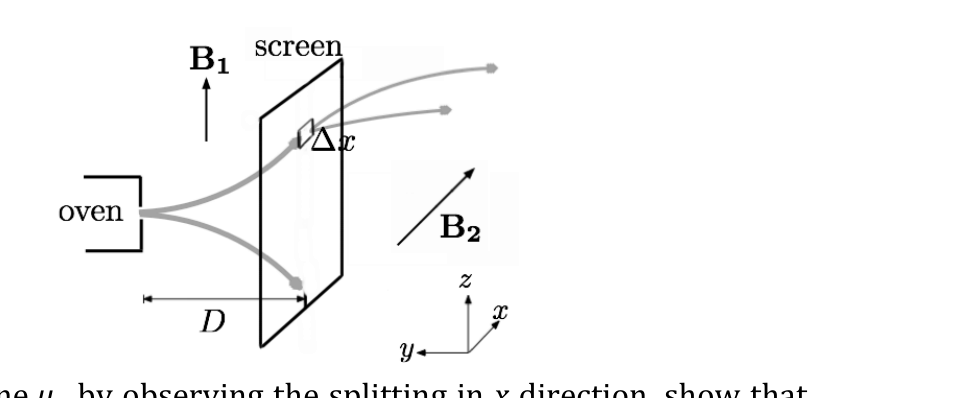
In order to determine ${\mu }_x$ by observing the splitting in $x$ direction, show that the following condition must be fulfilled: $\frac{1}{\hslash }|{\mu }_x|\Delta xCt\gg 1,$ where $t$ is the duration after leaving the screen $S{C}_1$ and $\Delta x$ is the opening width on $S{C}_1$.

2. (1.0 pts) The atoms are initially prepared in the spin up states right after leaving the screen, where ${\mu }_z=\gamma \hslash =|{\mu }_x|$. This means the atoms will precess at rates covering a range of values $\Delta \omega$ with respect to the $x$ component of ${\mathbf{B}}_2$, specifically $B_{2x}=B_0+Cx$. Prove that the spread in the precession angle $\Delta \omega t$ is so large and hence we cannot measure both ${\mu }_x$ and ${\mu }_z$ simultaneously. In other words, the measurement of ${\mu }_x$ destroys the information on ${\mu }_z$.

Fonte: Testo (PDF) — p.1

Topic: Magnetism, Modern-Quantum Physics Metodi: Torque & Angular Momentum Analysis, Differential Equations, Symmetry Argument, Vector Decomposition Competenze: Mathematical Modeling, Physical Reasoning Objects: Atom

Fisica del spin

Tutta la materia nell’universo ha proprietà fondamentali chiamate spin, oltre alla loro massa e carica. La rotazione è una forma intrinseca di impulso angolare trasportata dalle particelle. Nonostante il fatto che la meccanica quantistica sia necessaria per un completo trattamento dello spin, possiamo ancora studiare la fisica dello spin utilizzando il solito formalismo classico. In questo problema, stiamo studiando l’influenza del campo magnetico sul spin utilizzando il suo analogo classico.

L’equazione classica della coppia di spin è data da $\mathbf{\tau }=\frac{d\mathbf{L}}{dt}=\mathbf{\mu }\times \mathbf{B}.$ In questo caso, il momento angolare $\mathbf{L}$ rappresenta il spin “intrinseco” delle particelle, $\mathbf{\mu }$ è il momento magnetico delle particelle e $\mathbf{B}$ è il campo magnetico. Il spin di una particella è associato a un momento magnetico attraverso l’equazione $\mathbf{\mu }=-\gamma \mathbf{L}$ dove $\gamma$ è il rapporto giromagnetico.

In questo problema, il termine “frequenza” significa frequenza angolare (rad/s), che è una quantità scalare. Tutte le lettere in grasso rappresentano vettori; altrimenti rappresentano scalari.

Parte A. Precessione di Larmor (1,6 punti)

1. **(0,8 pts) ** Dimostra che la magnitudine del momento magnetico $\mu$ è sempre costante sotto l’influenza di un campo magnetico $\mathbf{B}$. Per un caso speciale di campo magnetico stazionario (constantino), indicare anche che l’angolo tra $\mathbf{\mu }$ e $\mathbf{B}$ è costante. (Signore: puoi usare le proprietà dei prodotti vettoriali.)

2. **(0,8 pts) ** Esiste un campo magnetico uniforme $\mathbf{B}$ che produce un angolo $\varphi$ con il momento magnetico di una particella $\mathbf{\mu }$. A causa della coppia del campo magnetico, il momento magnetico $\mathbf{\mu }$ ruota intorno al campo $\mathbf{B}$, noto anche come precessione di Larmor. Determinare la frequenza di precisione di Larmor ${\omega }_0$ del momento magnetico rispetto a $\mathbf{B}=B_0\mathbf{k}$.

Parte B. Quadro rotativo (3,4 punti)

In questa sezione, scegliamo un quadro rotativo $S^{\prime }$ come nostro quadro di riferimento. Il telaio rotante $S^{\prime }=(x^{\prime },y^{\prime },z^{\prime })$ ruota con una velocità angolare $\omega \mathbf{k}$ osservata da un osservatore nel telaio di laboratorio $S=(x,y,z)$, dove gli assi $x^{\prime },y^{\prime },z^{\prime }$ si intersecano con $x,y,z$ al tempo $t=0$. Qualsiasi vettore $\mathbf{A}=A_x\mathbf{i}+A_y\mathbf{j}+A_z\mathbf{k}$ in un quadro di laboratorio può essere scritto come $\mathbf{A}=A_{x^{\prime }}{\mathbf{i}}^{\prime }+A_{y^{\prime }}{\mathbf{j}}^{\prime }+A_{z^{\prime }}{\mathbf{k}}^{\prime }$ nel quadro di rotazione $S^{\prime }$. La derivata temporale del vettore diventa $\frac{d\mathbf{A}}{dt}=\frac{d{A}_{x^{\prime }}}{dt}{\mathbf{i}}^{\prime }+\frac{d{A}_{y^{\prime }}}{dt}{\mathbf{j}}^{\prime }+\frac{d{A}_{z^{\prime }}}{dt}{\mathbf{k}}^{\prime }+A_{x^{\prime }}\frac{d{\mathbf{i}}^{\prime }}{dt}+A_{y^{\prime }}\frac{d{\mathbf{j}}^{\prime }}{dt}+A_{z^{\prime }}\frac{d{\mathbf{k}}^{\prime }}{dt}$ ${\left(\frac{d\mathbf{A}}{dt}\right)}_{\mathrm{lab}}={\left(\frac{d\mathbf{A}}{dt}\right)}_{\mathrm{rot}}+\omega \mathbf{k}\times \mathbf{A},$ dove ${\left(\frac{d\mathbf{A}}{dt}\right)}_{\mathrm{lab}}$ è la derivata temporale del vettore $\mathbf{A}$ osservato da un osservatore nel quadro di laboratorio, e ${\left(\frac{d\mathbf{A}}{dt}\right)}_{\mathrm{rot}}$ è la derivata temporale osservata da un osservatore nel quadro di rotazione. Per tutti i seguenti problemi di questa parte, le risposte sono riportate nel quadro rotativo $S^{\prime }$.

1. **(0,8 pts) ** Mostra che l’evoluzione temporale del momento magnetico segue l’equazione ${\left(\frac{d\mathbf{\mu }}{dt}\right)}_{\mathrm{rot}}=-\gamma \mathbf{\mu }\times {\mathbf{B}}_{\mathrm{eff}},$ dove ${\mathbf{B}}_{\mathrm{eff}}=\mathbf{B}-\frac{\omega }{\gamma }{\mathbf{k}}^{\prime }$ è il campo magnetico effettivo.

2. **(0,4 pts) ** Per $\mathbf{B}=B_0\mathbf{k}$, qual è la nuova frequenza di precisione $\Delta$ in termini di ${\omega }_0$ e $\omega$?

3. **(1.2 pts) ** Ora, consideriamo il caso di un campo magnetico variabile nel tempo. Oltre a un campo magnetico costante, applichiamo anche un campo magnetico rotante $\mathbf{b}(t)=b(\cos \omega t\mathbf{i}+\sin \omega t\mathbf{j})$, quindi $\mathbf{B}=B_0\mathbf{k}+\mathbf{b}(t)$. Mostrare che la nuova frequenza di precisione di Larmor del momento magnetico è $\Omega =\gamma \sqrt{{\left(B_0-\frac{\omega }{\gamma }\right)}^2+b^2}.$

4. Invece di applicare il campo $\mathbf{b}(t)=b(\cos \omega t\mathbf{i}+\sin \omega t\mathbf{j})$, ora applichiamo $\mathbf{b}(t)=b(\cos \omega t\mathbf{i}-\sin \omega t\mathbf{j})$, che ruota nella direzione opposta e quindi $\mathbf{B}=B_0\mathbf{k}+b(\cos \omega t\mathbf{i}-\sin \omega t\mathbf{j})$. Qual è il campo magnetico efficace ${\mathbf{B}}_{\mathrm{eff}}$ per questo caso (in termini di vettori unitari ${\mathbf{i}}^{\prime },{\mathbf{j}}^{\prime },{\mathbf{k}}^{\prime }$)? Qual è la sua media temporale, $\overline{{\mathbf{B}}_{\mathrm{eff}}}$ (ricordate che $\overline{\cos 2\pi t/T}=\overline{\sin 2\pi t/T}=0$)?

Parte C. Oscillazione di Rabi (3,0 punti)

Per un insieme di particelle $N$ sotto l’influenza di un grande campo magnetico, lo spin può avere due stati quantistici: “alto” e “in basso”. Di conseguenza, la popolazione totale di spin up $N_{\uparrow }$ e down $N_{\downarrow }$ obbedisce all’equazione $N_{\uparrow }+N_{\downarrow }=N.$ La differenza tra popolazione spin up e popolazione spin down produce la magnetizzazione macroscopica lungo l’asse $z$: $M=(N_{\uparrow }-N_{\downarrow })\mu =N{\mu }_z.$ In un esperimento reale, di solito vengono applicati due campi magnetici, un campo di bias grande $B_0\mathbf{k}$ e un campo oscillante con amplitudine $2b$ perpendicolare al campo di bias ($b\ll B_0$). Inizialmente viene applicato solo il grande bias, causando che tutte le particelle si trovino negli stati di spin up ($\mathbf{\mu }$ è orientata nella direzione $z$ a $t=0$). In seguito, il campo oscillante viene attivato, dove la sua frequenza $\omega$ viene scelto per essere in risonanza con la frequenza di precisione di Larmor ${\omega }_0$, cioè $\omega ={\omega }_0$. In altre parole, il campo totale dopo il tempo $t=0$ è dato da $\mathbf{B}(t)=B_0\mathbf{k}+2b\cos {\omega }_{0}t\mathbf{i}.$

1. **(1.2 pts) ** Nel quadro rotativo $S^{\prime }$, mostrare che il campo effettivo può essere approssimato da ${\mathbf{B}}_{\mathrm{eff}}\approx b{\mathbf{i}}^{\prime },$ che è comunemente conosciuta come approssimazione delle onde rotanti. Qual è la frequenza di precisione $\Omega$ nel quadro $S^{\prime }$?

2. **(0,6 pts) ** Determina l’angolo $\alpha$ che $\mathbf{\mu }$ fa con ${\mathbf{B}}_{\mathrm{eff}}$. Inoltre, dimostrare che la magnetizzazione varia con il tempo come $M(t)=N\mu \cos \Omega t.$

3. **(1.2 pts) ** Con l’applicazione del campo magnetico descritto sopra, determinare la popolazione frazionaria di ogni spin su $P_{\uparrow }=N_{\uparrow }/N$ e spin verso il basso $P_{\downarrow }=N_{\downarrow }/N$ in funzione del tempo. Il plot $P_{\uparrow }(t)$ e $P_{\downarrow }(t)$ sullo stesso grafico vs. tempo $t$. La rotazione alterna in alto e in basso della popolazione in funzione del tempo si chiama oscillazione Rabi.

Parte D. Incompatibilità della misurazione (2,0 punti)

Spin è infatti una quantità vettoriale; ma a causa delle sue proprietà quantistiche, non possiamo misurare ogni componente contemporaneamente (cioè Possiamo conoscere sia $|\mathbf{\mu }|$ che ${\mu }_z$ come nei problemi precedenti; ma non tutti $|\mathbf{\mu }|,{\mu }_x,{\mu }_y,$ e ${\mu }_z$ contemporaneamente). In questo problema, faremo un calcolo basato sul principio di incertezza di Heisenberg (usando la relazione $\Delta p_q\Delta q\ge \hslash$) per mostrare come queste misurazioni siano incompatibili tra loro.

1. **(1.0 pts) ** Consideriamo una fonte di forno di atomi d’argento, che ha una piccola apertura. Gli atomi scorrono dall’apertura lungo la direzione $-y$ (vedi figura seguente) e sperimentano un campo variabile spaziale ${\mathbf{B}}_1$. Il campo ${\mathbf{B}}_1$ ha una componente di campo di forte bias nella direzione $z$, dove gli atomi con un momento magnetico diverso ${\mu }_z=\pm \gamma \hslash$ sono divisi nella direzione $z$. A distanza $D$ dalla fonte del forno, si pone uno schermo $S{C}_1$ che permetta di passare solo gli atomi a spin (bloccando gli atomi a spin down). Così, all’istante dopo aver superato lo schermo, gli atomi sono preparati in stati di spin up. Dopo lo schermo, gli atomi entrano in una regione di campo non omogeneo ${\mathbf{B}}_2$ dove gli atomi percepiscono una forza $F_x={\mu }_{x}C.$ Il campo ${\mathbf{B}}_2$ ha una componente di campo di forte bias nella direzione $x$, dove gli atomi hanno il momento magnetico ${\mu }_x=\pm \gamma \hslash$.

Per determinare ${\mu }_x$ osservando la divisione in direzione $x$, dimostrare che la seguente condizione deve essere soddisfatta: $\frac{1}{\hslash }|{\mu }_x|\Delta xCt\gg 1,$ dove $t$ è la durata dopo aver lasciato lo schermo $S{C}_1$ e $\Delta x$ è la larghezza di apertura su $S{C}_1$.

2. **(1.0 pts) ** Gli atomi sono inizialmente preparati nello stato di spin up subito dopo aver lasciato lo schermo, dove ${\mu }_z=\gamma \hslash =|{\mu }_x|$. Ciò significa che gli atomi precesseranno a velocità che coprono una gamma di valori $\Delta \omega$ rispetto alla componente $x$ di ${\mathbf{B}}_2$, in particolare $B_{2x}=B_0+Cx$. Prove che lo spread nell’angolo di precisione $\Delta \omega t$ è così grande e quindi non possiamo misurare simultaneamente ${\mu }_x$ e ${\mu }_z$. In altre parole, la misurazione di ${\mu }_x$ distrugge le informazioni su ${\mu }_z$.

Fonte: Testo (PDF) — p.1

Topic: Magnetism, Modern-Quantum Physics Metodi: Torque & Angular Momentum Analysis, Differential Equations, Symmetry Argument, Vector Decomposition Competenze: Mathematical Modeling, Physical Reasoning Objects: Atom