APhO 2015 — Teorica

The fractional quantum Hall effect (FQHE)

The fractional quantum Hall effect (FQHE) was discovered by D. C. Tsui and H. Stormer at Bell Labs in 1981. In the experiment electrons were confined in two dimensions on the GaAs side by the interface potential of a GaAs/AlGaAs heterojunction fabricated by A. C. Gossard (here we neglect the thickness of the two-dimensional electron layer). A strong uniform magnetic field $B$ was applied perpendicular to the two-dimensional electron system. As illustrated in Figure 1, when a current $I$ was passing through the sample, the voltage $V_H$ across the current path exhibited an unexpected quantized plateau (corresponding to a Hall resistance $R_H=3h/e^2$) at sufficiently low temperatures. The appearance of the plateau would imply the presence of fractionally charged quasiparticles in the system, which we analyze below. For simplicity, we neglect the scattering of the electrons by random potential, as well as the electron spin.

(a) In a classical model, two-dimensional electrons behave like charged billiard balls on a table. In the GaAs/AlGaAs sample, however, the mass of the electrons is reduced to an effective mass $m^{\ast }$ due to their interaction with ions.

(i) (2 point) Write down the equation of motion of an electron in perpendicular electric field $\vec{E}=-E_y\hat{y}$ and magnetic field $\vec{B}=B\hat{z}$.

(ii) (1 point) Determine the velocity $v_s$ of the electrons in the stationary case.

(iii) (1 point) Which direction is the velocity pointing at?

(b) (2 points) The Hall resistance is defined as $R_H=V_H/I$. In the classical model, find $R_H$ as a function of the number of the electrons $N$ and the magnetic flux $\varphi =BWL$, where $A$ is the area of the sample, and $W$ and $L$ the effective width and length of the sample, respectively.

(c) (2 points) We know that electrons move in circular orbits in the magnetic field. In the quantum mechanical picture, the impinging magnetic field $B$ could be viewed as creating tiny whirlpools, so-called vortices, in the sea of electrons — one whirlpool for each flux quantum $h/e$ of the magnetic field. For the case of $R_H=3h/e^2$, which was discovered by Tsui and Stormer, derive the ratio of the number of the electrons $N$ to the number of the flux quanta $N_{\varphi }$, known as the filling factor $\nu$.

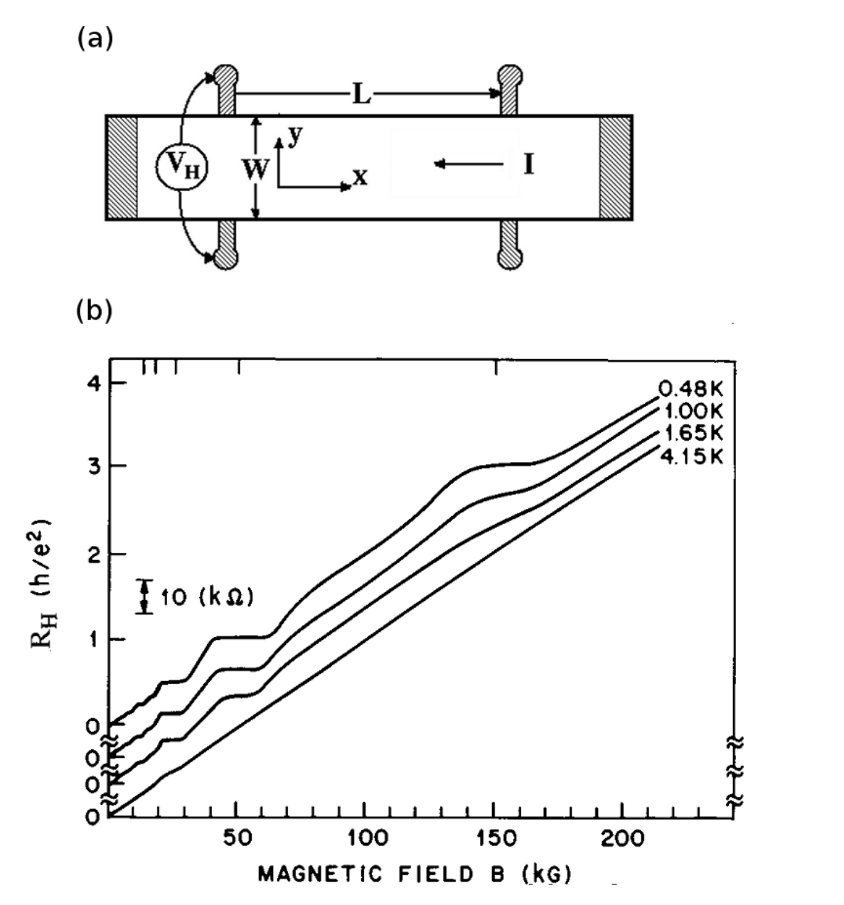
Figure 1: (a) Sketch of the experimental setup for the observation of the FQHE. As indicated, a current $I$ is passing through a two-dimensional electron system in the longitudinal direction with an effective length $L$. The Hall voltage $V_H$ is measured in the transverse direction with an effective width $W$. In addition, a uniform magnetic field $B$ is applied perpendicular to the plane. The direction of the current is given for illustrative purpose only, which may not be correct. (b) Hall resistance $R_H$ versus $B$ at four different temperatures (curves shifted for clarity) in the original publication on the FQHE. The features at $R_H=3h/e^2$ are due to the FQHE.

(d) (2 points) It turns out that binding an integer number of vortices ($n>1$) with each electron generates a bigger surrounding whirlpool, hence pushes away all other electrons. Therefore, the system can considerably reduce its electrostatic Coulomb energy at the corresponding filling factor. Determine the scaling exponent $\alpha$ of the amount of energy gain for each electron $\Delta U(B)\propto B^{\alpha }$.

(e) (2 points) As the magnetic field deviates from the exact filling $\nu =1/n$ to a higher field, more vortices (whirlpools in the electron sea) are being created. They are not bound to electrons and behave like particles carrying effectively positive charges, hence known as quasiholes, compared to the negatively charged electrons. The amount of charge deficit in any of these quasiholes amounts to exactly $1/n$ of an electronic charge. An analogous argument can be made for magnetic fields slightly below $\nu$ and the creation of quasielectrons of negative charge $e^{\ast }=-e/n$. At the quantized Hall plateau of $R_H=3h/e^2$, calculate the amount of change in $B$ that corresponds to the introduction of exactly one fractionally charged quasihole. (When their density is low, the quasiparticles are confined by the random potential generated by impurities and imperfections, hence the Hall resistance remains quantized for a finite range of $B$.)

(f) In Tsui et al. experiment, the magnetic field corresponding to the center of the quantized Hall plateau is

$R_H=3h/e^2,B_{1/3}=15\text{Tesla}.$

the effective mass of an electron in GaAs, $m^{\ast }=0.067m_e$,

the electron mass, $m_e=9.1\times 10^{-31}$ kg,

Coulomb’s constant, $k=9.0\times 10^9\text{N}\cdot {\text{m}}^2/{\text{C}}^2$,

the vacuum permittivity, ${\epsilon }_0=1/4\pi k=8.854\times 10^{-12}$ F/m,

the relative permittivity (the ratio of the permittivity of a substance to the vacuum permittivity) of GaAs, ${\epsilon }_r=13$,

the elementary charge, $e=1.6\times 10^{-19}$ C,

Planck’s constant, $h=6.626\times 10^{-34}$ J·s,

Boltzmann’s constant, $k_B=1.38\times 10^{-23}$ J/K.

In our analysis, we have neglected several factors, whose corresponding energy scales, compared to $\Delta U(B)$ discussed in (d), are either too large to excite or too small to be relevant.

(i) (1 point) Calculate the thermal energy $E_{th}$ at temperature $T=1.0$ K.

(ii) (2 points) The electrons spatially confined in the whirlpools (or vortices) have a large kinetic energy. Using the uncertainty relation, estimate the order of magnitude of the kinetic energy $E_k$ of such an electron. (This amount would also be the additional energy penalty if we put two electrons in the same whirlpool, instead of in two separate whirlpools, due to Pauli exclusion principle.)

(g) There are also a series of plateaus at $R_H=h/i{e}^2$, where $i=1,2,3,\dots$ in Tsui et al. experiment, as shown in Figure 1(b). These plateaus, known as the integer quantum Hall effect (IQHE), were reported previously by K. von Klitzing in 1980. Repeating (c)-(f) for the integer plateaus, one realizes that the novelty of the FQHE lies critically in the existence of fractionally charged quasiparticles, $R$.

Fonte: Testo (PDF) — p.1

Topic: Modern-Quantum Physics, Magnetism Metodi: Lorentz Force Analysis, Bohr Model & Quantization, Order-of-Magnitude Estimation, Photon Energy Relation Competenze: Physical Reasoning, Estimation & Approximation Objects: Electron

**L’effetto Hall quantistico frazionato (FQHE) **

L’effetto Hall quantistico frazionario (FQHE) è stato scoperto da D. C. Tsui e H. Stormer al Bell Labs nel 1981. Nell’esperimento gli elettroni sono stati confinati in due dimensioni sul lato delle GaAs dal potenziale di interfaccia di un eterogeno GaAs/AlGaAs fabbricato da A. C. Gossard (qui si trascura lo spessore dello strato elettronica bidimensionale). Un forte campo magnetico uniforme $B$ è stato applicato perpendicolare al sistema di elettroni bidimensionali. Come illustrato nella figura 1, quando un corrente $I$ passava attraverso il campione, la tensione $V_H$ lungo il percorso corrente presentava un inaspettato piano quantizzato (corrispondente a una resistenza Hall $R_H=3h/e^2$) a temperature sufficientemente basse. L’aspetto dell’altopiano implicerebbe la presenza di quasiparticelle frazionatamente cariche nel sistema, che analizziamo di seguito. Per semplicità, trascuriamo la dispersione degli elettroni da potenziale casuale, così come lo spin degli elettroni.

In un modello classico, gli elettroni bidimensionali si comportano come palline di biliardo cariche su un tavolo. Nel campione GaAs/AlGaAs, tuttavia, la massa degli elettroni è ridotta a una massa effettiva $m^{\ast }$ a causa della loro interazione con gli ioni.

(i) **(2 punto) ** Scrivere l’equazione del movimento di un elettrone nel campo elettrico perpendicolare $\vec{E}=-E_y\hat{y}$ e nel campo magnetico $\vec{B}=B\hat{z}$.

(ii) **(1 punto) ** Determina la velocità $v_s$ degli elettroni nel caso stazionario.

(iii) **1 punto) ** In quale direzione punta la velocità?

**(b) ** **(2 punti) ** La resistenza Hall è definita come $R_H=V_H/I$. Nel modello classico, trovare $R_H$ come funzione del numero di elettroni $N$ e del flusso magnetico $\varphi =BWL$, dove $A$ è l’area del campione, e $W$ e $L$ rispettivamente la larghezza e la lunghezza effettive del campione.

**(c) ** **(2 punti) ** Sappiamo che gli elettroni si muovono in orbite circolari nel campo magnetico. Nell’immagine meccanica quantistica, il campo magnetico impingente $B$ potrebbe essere visto come la creazione di piccoli turbolini, i cosiddetti vortici, nel mare di elettroni un turbolino per ogni flusso quantistico $h/e$ del campo magnetico. Per il caso di $R_H=3h/e^2$, scoperto da Tsui e Stormer, derivare il rapporto tra il numero di elettroni $N$ e il numero dei quanti di flusso $N_{\varphi }$, noto come fattore di riempimento $\nu$.

Figura 1: a) Sketto dell’impianto sperimentale per l’osservazione della FQHE. Come indicato, una corrente $I$ passa attraverso un sistema di elettroni bidimensionali nella direzione longitudinale con una lunghezza effettiva $L$. La tensione di Hall $V_H$ è misurata in direzione trasversale con una larghezza effettiva $W$. Inoltre, viene applicato un campo magnetico uniforme $B$ perpendicolare al piano. La direzione della corrente è data solo per scopi illustrativi, che potrebbero non essere corretti. b) Resistenza di sala $R_H$ rispetto a $B$ a quattro temperature diverse (corve spostate per la chiarezza) nella pubblicazione originale sul FQHE. Le caratteristiche di $R_H=3h/e^2$ sono dovute alla FQHE.

**(d) ** **(2 punti) ** Si scopre che legare un numero intero di vortici ($n>1$) con ogni elettrone genera un urlo più grande circostante, spingendo quindi via tutti gli altri elettroni. Pertanto, il sistema può ridurre notevolmente la sua energia elettrostatica di Coulomb al corrispondente fattore di riempimento. Determinare l’esponente di scalazione $\alpha$ della quantità di guadagno energetico per ogni elettrone $\Delta U(B)\propto B^{\alpha }$.

**(e) ** **(2 punti) ** Mentre il campo magnetico si allontana dall’esatto riempimento $\nu =1/n$ a un campo più alto, si creano più vortici (torcicoli nel mare di elettroni). Non sono legati agli elettroni e si comportano come particelle che portano cariche positive efficacemente, quindi conosciute come quasi-buchi, rispetto agli elettroni carichi negativamente. L’importo del deficit di carico in uno di questi quasi-pericoli è esattamente $1/n$ di un carico elettronico. Un argomento analogo può essere fatto per campi magnetici leggermente inferiori a $\nu$ e la creazione di quasielettroni di carica negativa $e^{\ast }=-e/n$. Al piano di Hall quantizzato di $R_H=3h/e^2$, calcolare la quantità di variazione in $B$ che corrisponde all’introduzione di esattamente un quasi-luco carico frazionalmente. (Quando la loro densità è bassa, le quasiparticelle sono confinate dal potenziale casuale generato da impurità e imperfezioni, quindi la resistenza di Hall rimane quantizzata per un intervallo finito di $B$.)

In questo esperimento, il campo magnetico corrispondente al centro del piatto Hall quantizzato è:

$R_H=3h/e^2,B_{1/3}=15\text{Tesla}.$

la massa effettiva di un elettrone in GaAs, $m^{\ast }=0.067m_e$,

la massa degli elettroni, $m_e=9.1\times 10^{-31}$ kg,

Costante di Coulomb, $k=9.0\times 10^9\text{N}\cdot {\text{m}}^2/{\text{C}}^2$,

la capacità di scarico del vuoto, ${\epsilon }_0=1/4\pi k=8.854\times 10^{-12}$ F/m,

la relativa permissività (il rapporto tra la permissività di una sostanza e la permissività al vuoto) di GaAs, ${\epsilon }_r=13$,

la carica elementare, $e=1.6\times 10^{-19}$ C,

Costante di Planck, $h=6.626\times 10^{-34}$ J·s,

Costante di Boltzmann, $k_B=1.38\times 10^{-23}$ J/K.

Nella nostra analisi abbiamo trascurato diversi fattori, le cui scale energetiche corrispondenti, rispetto a $\Delta U(B)$ discusse nella lettera d), sono troppo grandi per eccitare o troppo piccole per essere rilevanti.

(i) **(1 punto) ** Calcolare l’energia termica $E_{th}$ a temperatura $T=1.0$ K.

(ii) **(2 punti) ** Gli elettroni confinati spazialmente nei turbolini (o vortici) hanno una grande energia cinetica. Utilizzando la relazione di incertezza, stimare l’ordine di grandezza dell’energia cinetica $E_k$ di un tale elettrone. (Questa quantità sarebbe anche la penalità di energia aggiuntiva se mettiamo due elettroni nello stesso turbolino, invece di due turbolini separati, a causa del principio di esclusione di Pauli.)

**(g) ** Ci sono anche una serie di altopiani a $R_H=h/i{e}^2$, dove $i=1,2,3,\dots$ in Tsui et al. esperimento, come mostrato nella Figura 1(b). Questi pianeti, noti come effetto Hall quantistico interi (IQHE), sono stati precedentemente riportati da K. Von Klitzing nel 1980. Ripetendo (c) - (f) per gli altopiani interi, si capisce che la novità della FQHE risiede criticamente nell’esistenza di quasiparticelle cariche frazionalmente, $R$.

Fonte: Testo (PDF) — p.1

Topic: Modern-Quantum Physics, Magnetism Metodi: Lorentz Force Analysis, Bohr Model & Quantization, Order-of-Magnitude Estimation, Photon Energy Relation Competenze: Physical Reasoning, Estimation & Approximation Objects: Electron

How are aurora ignited by the solar wind?

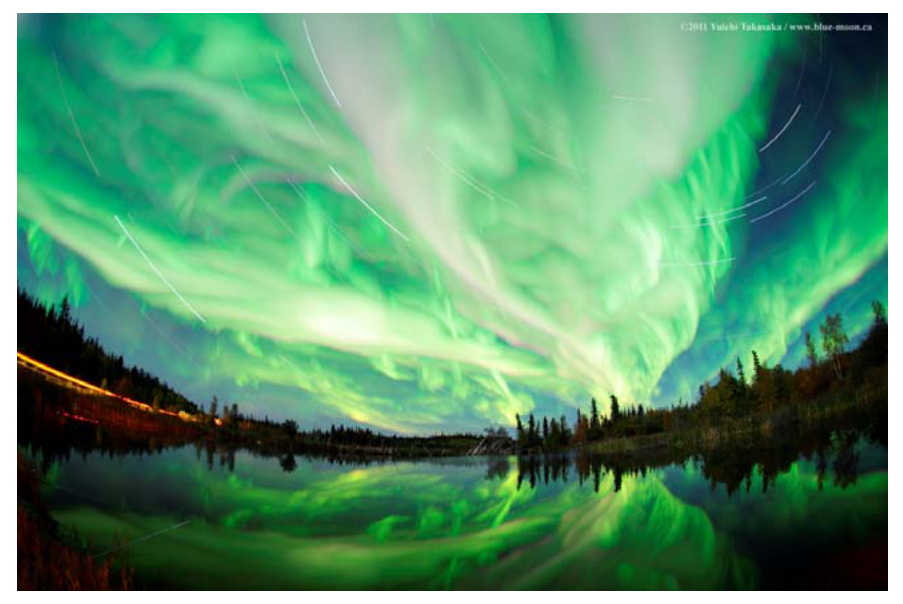
Figure 1

The following questions are designed to guide you to find the answer one step by one step.

Background information of the interaction between the solar wind and the Earth’s magnetic field

It is well known that the Earth has a substantial magnetic field. The field lines defining the structure of the Earth’s magnetic field is similar to that of a simple bar magnet, as shown in Figure 2. The Earth’s magnetic field is disturbed by the solar wind, whichis a high-speed stream of hot plasma. (The plasma is the quasi-neutralionized gas.)The plasma blows outward from the Sun and varies in intensity with the amount of surface activity on the Sun. The solar wind compresses the Earth’s magnetic field. On the other hand, the Earth’s magnetic field shields the Earth from much of the solar wind. When the solar wind encounters the Earth’s magnetic field, it is deflected like water around the bow of a ship, as illustrated in Figure 3.

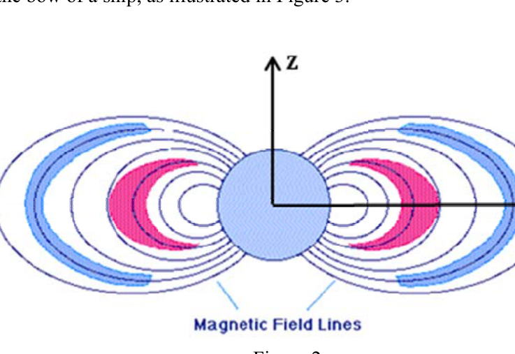
Figure 2

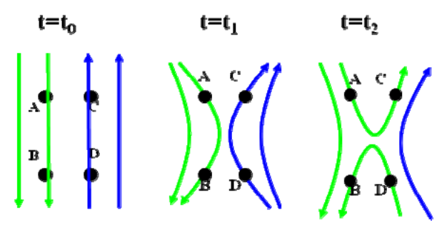
The curved surface at which the solar wind is first deflected is called the bow shock. The corresponding region behind the bow shock andfront of the Earth’s magnetic field is called the magnetosheath. The region surroundedby the solar wind is called the magnetosphere.The Earth’s magnetic field largely prevents the solar wind from enteringthe magnetosphere. The contact region between the solar wind and the Earth’s magnetic field is named the magnetopause. The location of the magnetopause is mainly determined by the intensity and the magnetic field direction of the solar wind. When the magnetic field in the solar wind is antiparallel to the Earth’s magnetic field, magnetic reconnection as shown in Figure 4 takes place at the dayside magnetopause, which allows charged particles enter into the magnetosphere. The ‘point A’ marked in the magnetopause, which means charged particles offthe solar wind enter into the magnetosphere, is the region “A” to move into the region “P”. The energetic particles in the solar wind couldcause high-transfer of magnitude of the kinetic energy. (This amount would also be the additional energy penalty if we put two electrons in the same whirlpool, instead of in two separate whirlpools due to Pauli exclusion principle?)

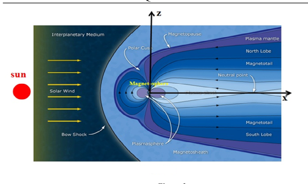
Figure 3

we first considerthe motion of an electron in a uniform magnetic field $\vec{B}$. When the initial electron velocity $\vec{v}$ is perpendicular to the uniform magnetic field as shown in Figure 6, please calculate the electron trajectory.The electron is initially located at $(x,y,z)=(0,0,0)$.

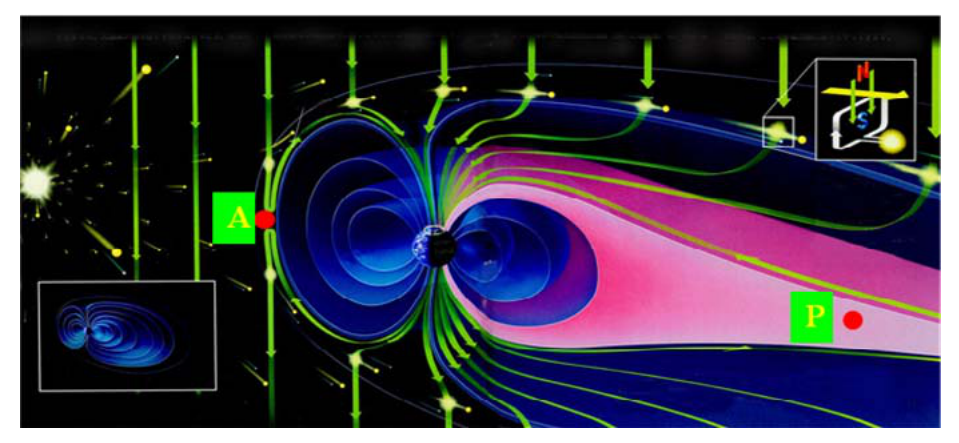
Figure 5

Numerical values of physical constants and the Earth’s dipole magnetic field:

Speed of light in vacuum: $c=2.998\times 10^8\text{m/s}$;

Permittivity in vacuum: ${\epsilon }_0=8.9\times 10^{-12}{\text{C}}^2/(\text{N}\cdot {\text{m}}^2)$;

Permeability in vacuum: ${\mu }_0=4\pi \times 10^{-7}{\text{N/A}}^2$;

Charge of a proton: $e=1.6\times 10^{-19}$ C;

Mass of an electron: $m=9.1\times 10^{-31}$ kg;

Mass of a proton: $m_p=1.67\times 10^{-27}$ kg;

Boltzmann’s constant: $k=1.38\times 10^{-23}$ J/K;

Gravitational acceleration: $g=9.8{\text{m/s}}^2$;

Planck’s constant: $h=6.626\times 10^{-34}$ J·s;

Earth’s radius: $R_E=6.4\times 10^6$ m.

The Earth’s dipole magnetic field can be expressed as

\vec{B}_d = \frac{B_0 R_0^3}{r^5}\left[3xz\hat{x} - 3yz\hat{y} + (x^2 + y^2 - 2z^2)\hat{z}\right],\quad (r \ge R_0)\tag{1}

where $r=\sqrt{x^2+y^2+z^2}$, $B_0=3.1\times 10^{-5}$ T, and $\hat{x},\hat{y},\hat{z}$ are the unit vectors in the $x,y,z$ directions, respectively.

Questions:

(a) (3 Points)

(i) (1 Point) Before we study the motion of a charged particle in the Earth’s dipole magnetic field, we first considerthe motion of an electron in a uniform magnetic field $\vec{B}$. When the initial electron velocity $\vec{v}$ is perpendicular to the uniform magnetic field as shown in Figure 6, please calculate the electron trajectory.The electron is initially located at $(x,y,z)=(0,0,0)$.

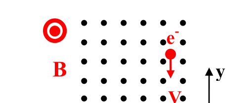
Figure 6

(ii) (1 Point) Please determine the electric current of the electron motion and calculate the magnetic moment $\vec{\mu }=i\vec{A}$, where $\vec{A}$ is the area of the electron circular orbit and the direction of $\vec{A}$ is determined by the right-hand rule of theelectric current.

(iii) (1 Point) If the initial electron velocity $\vec{v}$ is not perpendicular to the uniform magnetic field, i.e, the angle $\theta$ between $\vec{B}$ and $\vec{v}$ is $0°<\theta <90°$, please give the screw pitch (the distance along the $z$-axis between successive orbits) of the electron trajectory.

(b) (4 Points) In the uniform background magnetic field as shown in Figure 6, theplasma density isnonuniform in $x$. For simplicity, we assume that the temperature and the distribution of the ions andelectrons are the same. Thus, the plasma pressure can be expressed as

$p(x)=kT[n_i(x)+n_e(x)]=2kTn(x)=2kT(n_0+\alpha x),$

Where $B,T,k,n_0$, and $\alpha$ are positive constants, $n_i(x)$ and $n_e(x)$ are the number densities of the ions and electrons.

(i) (2 points) Please explain the generation mechanism of the electric current by a schematic drawing.

(ii) (2 points) If both the ions and electrons have a Maxwellian distribution, the ion distribution is

$f_i(x,v_x,v_y)=n_i(x){\left(\frac{m_i}{2\pi kT}\right)}^{3/2}{e}^{-m_i(v_x^2+v_y^2)/2kT},$

please calculate the constant $\beta$ in the magnetization $M=\beta n(x)\frac{kT}{B}$, where the magnetization $M$is the magnetic moment per unit volume. (Hint: We have ${\int }_0^{\infty }x\exp (-x)dx=1$ and ${\int }_{-\infty }^{\infty }\exp (-x^2)dx=\sqrt{\pi }$.)

(c) **(1 Point)**Now let’s go back to the Earth’s dipole magnetic field. Please apply the result from Question(b) to calculate the ratio of the diamagnetic field and the Earth’s dipole magnetic field in Equation (1) at the position ($x=10R_0$, $y=0$, $z=1$ $R_0$). The plasma pressure is assumed to be

$p(z)=p_0{e}^{-z/z{\sigma }^2},\text{where }{p}_0=3\times 10^{-10}\text{pa}\text{ and }a=2R_E.$

The magnetic field around this position is also assumed to be uniform. Be aware of the difference in the coordinate systemin Questions (b) and (c). (Hint: The diamagnetic field is given by $B_{dia}={\mu }_{0}M$.)

(d) (4 Points) From Figures 2, 3, and 5, it can be clearly seen that the Earth’s magnetic fieldstrength along a magnetic field line is the largest at the poles and the smallest in the equatorial plane.Since the Earth’s dipole magnetic field is axially symmetric and slowly varying along a magnetic field line, it can for simplicitybe treated as a magnetic-mirror field as shown in Figure 7.The magnetic field strength along a magnetic field line is the smallest ($B_0$) at the point "$P_2$" and the largest ($B_m$) at the points "$P_1$" and "$P_3$". An electron with an initial velocity $\vec{v}$ is located at the point "$P_2$" and drifts towards the point "$P_1$". The angle between the initial velocity $\vec{v}$ and the magnetic field at the point "$P_2$" is $0°<\theta <90°$. For the magnetic-mirror field $\vec{B}=B_r\hat{r}+B_z\hat{z}$ (with $B_r<<B_z$), we can assume $\frac{dB}{dz}\approx \frac{dB}{ds}$, where $\frac{dB}{ds}$ is the spatial derivative of $B$ along a magnetic field line. Since there is no evidence of the existence of magnetic monopoles, we have $⟨B_r⟩=-\frac{1}{2}\frac{dB}{dz}{r}_c<<B_z$, where $⟨B_r⟩$ is the gyro-average of $B_r$ and $r_c$ is the electron gyroradius.

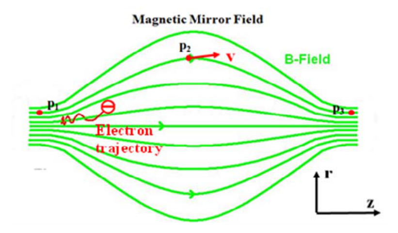
Figure 7

(i) (3 Points) Please givethe gyro-averaged magnetic field force along the magnetic field lines on an electron and show that the magnetic moment is a motion constant, i.e., $\frac{d\mu }{dt}=0$, based on the law of the total kinetic energy conservation.

(ii) (1 Point) Based on the motion constant of magnetic moment, please determinewhat the condition should be satisfied for the angle $\theta$ between the initial electron velocity $\vec{v}$ and the magnetic field at the point "$P_2$"(an electron will not escape from the magnetic mirror field.

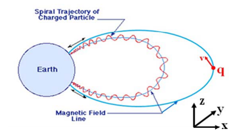
(e) (1 Point) Each magnetic field lines (blue lines) are shown in Figure 8. The spiral trajectory of a charged particle (red curve) is assumed to be confined in the $(x-y)$ plane since the gradient and the curvature of the magnetic field can be ignored. If a charged particle with the mass $m$, charge $q$, and velocity $\vec{v}$ is initially located at the equatorial point [$x=4R_E$, $y=0$, $z=0$] plane and drifts towards the positive $y$-axis where the magnetic field is $\theta$. Initially, please determine what the condition should be satisfied for $\theta$ if the charged particle arrives below 200km of its altitude at the latitude 60°.

(f) (5 Points) As shown in Figure 5, when magnetic reconnection takes place at the dayside magnetopause, reconnected magnetic field lines drift towards the nightside region because the solar wind flows tailward. Thus, some solar wind electrons in the region “A” also move towards the magnetotail in the region “P”. After the electrons arrive in the region “P”, some electrons can be accelerated to around 1keV. If energetic electrons drift down to the thermosphere (The altitude of the thermosphere is about 85km-800km.), energetic electrons can collide with the neutral atoms, which could cause the neutral atoms to jump into excited states. A photon is emitted when the higher excited state of aneutral atom returns to lower excited state or ground state. Splendid aurora (Figure 1) is generated in the aurora oval due to photons with different wavelengths. It is found that the aurorais mainly resulted fromphotonsemittedby oxygen atoms.The energy levels in the first and second excited states relative to the ground stateare 1.96eV and 4.17eV, respectively. The lifetimes of the two excited states of an oxygen atomare 110s and 0.8s as shown in Figure 9.

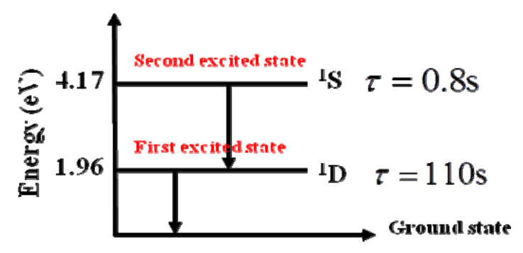
Figure 9

(i) (2 Points) Please give the atmospheric density as a function of the altitude and the ratio of the oxygen density at the altitudes H=160km and H=220km. For simplicity, we assume that the atmospheric temperature is independent of the altitude and the air is an ideal gas. (${\rho }_{a}g/P_a=0.13$ / km, where ${\rho }_a$ and $P_a$ the atmospheric density and pressure at sea level.)

(ii) **(2 Points)**Please give the colors of auroras at the altitudes H=160km and H=220km. (Hint: The collision frequency of the collision frequency of atmosphericmolecules at the atmospheric density is independent of the altitude and the air is an ideal gas. ${\nu }_c=v_{re}{\rho }_a/p_a$, where $v_0\approx 10^9$ /s is the collision frequency of atmosphericmolecules at sea level.The excited oxygen atom will lose a part of its energy when it collides with other neutral molecules.)

(g) (2 points) As mentioned above, a powerful solar wind can push the dayside magnetopause tovery close to the Earth, which could cause a high-orbit satelliteto be fully exposed to the solar wind. The energetic particles in the solar wind could damage high-tech electronic components in a satellite.For simplicity, the Earth’s dipole magnetic field is assumed to remain unchanged when the solar wind compresses it and that the plasma density is ignorable in the magnetosphere. Please give the minimum solar wind speed to cause a damage of a geosynchronous satellite if the magnetic field strength and the plasma density of the solar wind are $B_s=5\times 10^{-9}$ T and ${\rho }_s=50\text{proton}/{\text{cm}}^3$, respectively. (Hint: The force per unit area associated with the magnetic field is $f=B^2/2{\mu }_0$. We only consider the variation in $x$ for all physical quantities, i.e., the physical quantities are independent of $y$ and $z$.)

Fonte: Testo (PDF) — p.1

Topic: Magnetism, Earth & Environmental Science Metodi: Lorentz Force Analysis, Statistical Averaging, Hydrostatic Equilibrium, Conservation of Energy Competenze: Physical Reasoning, Mathematical Modeling Objects: Planet, Electron, Satellite, Magnet

How are aurora ignited by the solar wind?

Figura 1

Le seguenti domande sono progettate per aiutarti a trovare la risposta passo dopo passo.

Informazioni di base sull’interazione tra il vento solare e il campo magnetico terrestre

È noto che la Terra ha un campo magnetico sostanziale. Le linee di campo che definiscono la struttura del campo magnetico terrestre sono simili a quelle di un semplice magnete a barre, come mostrato nella Figura 2. Il campo magnetico terrestre è disturbato dal vento solare, che è un flusso ad alta velocità di plasma caldo. (Il plasma è il gas quasi neutralizzato.)Il plasma soffia verso l’esterno dal Sole e varia in intensità con la quantità di attività superficiale sul Sole. Il vento solare compresse il campo magnetico terrestre. D’altra parte, il campo magnetico terrestre protegge la Terra da gran parte del vento solare. Quando il vento solare incontra il campo magnetico terrestre, si devia come l’acqua intorno all’arco di una nave, come illustrato nella Figura 3.

Figura 2

La superficie curva in cui il vento solare viene deviato per la prima volta si chiama scossa dell’arco **. The corresponding region behind the bow shock andfront of the Earth’s magnetic field is called the magnetosheath. The region surroundedby the solar wind is called the magnetosphere.The Earth’s magnetic field largely prevents the solar wind from enteringthe magnetosphere. La regione di contatto tra il vento solare e il campo magnetico terrestre è chiamata magnetopause. La posizione della magnetopausa è determinata principalmente dall’intensità e dalla direzione del campo magnetico del vento solare. Quando il campo magnetico del vento solare è antiparallelle al campo magnetico terrestre, la riconnessione magnetica come mostrato nella figura 4 si verifica alla magnetopausa di giorno, che consente alle particelle cariche di entrare nella magnetosfera. Il “punto A” segnato nella magnetopausa, che significa particelle cariche del vento solare che entrano nella magnetosfera, è la regione “A” per spostarsi nella regione “P”. Le particelle energetiche del vento solare potrebbero causare un trasferimento di grandezza dell’energia cinetica. (Questa quantità sarebbe anche la penalità di energia aggiuntiva se mettiamo due elettroni nello stesso turbolino, invece di due turbolini separati a causa del principio di esclusione di Pauli?)

Figura 3

In primo luogo, consideriamo il movimento di un elettrone in un campo magnetico uniforme $\vec{B}$. When the initial electron velocity $\vec{v}$ is perpendicular to the uniform magnetic field as shown in Figure 6, please calculate the electron trajectory.The electron is initially located at $(x,y,z)=(0,0,0)$.

Figura 5

Valuti numerici delle costanti fisiche e del campo magnetico di dipole terrestre:

velocità della luce al vuoto: $c=2.998\times 10^8\text{m/s}$;

Permettività al vuoto: ${\epsilon }_0=8.9\times 10^{-12}{\text{C}}^2/(\text{N}\cdot {\text{m}}^2)$;

Permeabilità al vuoto: ${\mu }_0=4\pi \times 10^{-7}{\text{N/A}}^2$;

carico di un protone: $e=1.6\times 10^{-19}$ C;

Massa di un elettrone: $m=9.1\times 10^{-31}$ kg;

Massa di un protone: $m_p=1.67\times 10^{-27}$ kg;

Costante di Boltzmann: $k=1.38\times 10^{-23}$ J/K;

Accelerazione gravitazionale: $g=9.8{\text{m/s}}^2$;

Costante di Planck: $h=6.626\times 10^{-34}$ J·s;

Radius della Terra: $R_E=6.4\times 10^6$ m.

Il campo magnetico di dipole della Terra può essere espresso come

\vec{B}_d = \frac{B_0 R_0^3}{r^5}\left[3xz\hat{x} - 3yz\hat{y} + (x^2 + y^2 - 2z^2)\hat{z}\right],\quad (r \ge R_0)\tag{1}

dove $r=\sqrt{x^2+y^2+z^2}$, $B_0=3.1\times 10^{-5}$ T e $\hat{x},\hat{y},\hat{z}$ sono i vettori unitari nelle direzioni $x,y,z$, rispettivamente.

Domande:

**(a) ** **(3 punti) **

(i) (1 Point) Before we study the motion of a charged particle in the Earth’s dipole magnetic field, we first considerthe motion of an electron in a uniform magnetic field $\vec{B}$. When the initial electron velocity $\vec{v}$ is perpendicular to the uniform magnetic field as shown in Figure 6, please calculate the electron trajectory.The electron is initially located at $(x,y,z)=(0,0,0)$.

Figura 6

(ii) **(1 punto) ** Determina la corrente elettrica del movimento degli elettroni e calcola il momento magnetico $\vec{\mu }=i\vec{A}$, dove $\vec{A}$ è l’area dell’orbita circolare degli elettroni e la direzione di $\vec{A}$ è determinata dalla regola destra della corrente elettrica.

(iii) **(1 Punto) ** Se la velocità iniziale degli elettroni $\vec{v}$ non è perpendicolare al campo magnetico uniforme, cioè l’angolo $\theta$ tra $\vec{B}$ e $\vec{v}$ è $0°<\theta <90°$, indicare il punto di visatura (la distanza lungo l’asse $z$ tra le orbite successive) della traiettoria degli elettroni.

**(b) ** **(4 punti) ** Nel campo magnetico di fondo uniforme come illustrato nella figura 6, la densità plasmatica non è uniforme in $x$. Per semplicità, supponiamo che la temperatura e la distribuzione degli ioni e degli endelettoni siano uguali. La pressione plasmatica può quindi essere espressa come

$p(x)=kT[n_i(x)+n_e(x)]=2kTn(x)=2kT(n_0+\alpha x),$

Se $B,T,k,n_0$ e $\alpha$ sono costanti positive, $n_i(x)$ e $n_e(x)$ sono le densità numeriche degli ioni ed elettroni.

(i) **(2 punti) ** Per favore, spiegate il meccanismo di generazione della corrente elettrica mediante un disegno schematico.

(ii) **(2 punti) ** Se sia gli ioni che gli elettroni hanno una distribuzione maxwelliana, la distribuzione degli ioni è

$f_i(x,v_x,v_y)=n_i(x){\left(\frac{m_i}{2\pi kT}\right)}^{3/2}{e}^{-m_i(v_x^2+v_y^2)/2kT},$

Calcolare la costante $\beta$ nella magnetizzazione $M=\beta n(x)\frac{kT}{B}$, dove la magnetizzazione $M$ è il momento magnetico per unità di volume. (Signore: abbiamo ${\int }_0^{\infty }x\exp (-x)dx=1$ e ${\int }_{-\infty }^{\infty }\exp (-x^2)dx=\sqrt{\pi }$.)

(c) **(1 Point)**Now let’s go back to the Earth’s dipole magnetic field. Si prega di applicare il risultato della domanda ((b) per calcolare il rapporto tra il campo diamagnetico e il campo magnetico di dipole terrestre nell’equazione (1) alla posizione ($x=10R_0$, $y=0$, $z=1$ $R_0$). Si presume che la pressione plasmatica sia

$p(z)=p_0{e}^{-z/z{\sigma }^2},\text{where }{p}_0=3\times 10^{-10}\text{pa}\text{ and }a=2R_E.$

Si presume anche che il campo magnetico attorno a questa posizione sia uniforme. Si noti la differenza nel sistema di coordinate nelle domande (b) e (c). (Signore: il campo diamagnetico è dato da $B_{dia}={\mu }_{0}M$.)

(d) (4 Points) From Figures 2, 3, and 5, it can be clearly seen that the Earth’s magnetic fieldstrength along a magnetic field line is the largest at the poles and the smallest in the equatorial plane.Since the Earth’s dipole magnetic field is axially symmetric and slowly varying along a magnetic field line, it can for simplicitybe treated as a magnetic-mirror field as shown in Figure 7.The magnetic field strength along a magnetic field line is the smallest ($B_0$) at the point "$P_2$" and the largest ($B_m$) at the points "$P_1$" and "$P_3$". Un elettrone con una velocità iniziale $\vec{v}$ si trova al punto "$P_2$" e deriva verso il punto "$P_1$". L’angolo tra la velocità iniziale $\vec{v}$ e il campo magnetico al punto "$P_2$" è $0°<\theta <90°$. Per il campo di specchio magnetico $\vec{B}=B_r\hat{r}+B_z\hat{z}$ (con $B_r<<B_z$), possiamo assumere $\frac{dB}{dz}\approx \frac{dB}{ds}$, dove $\frac{dB}{ds}$ è la derivata spaziale di $B$ lungo una linea di campo magnetico. Poiché non ci sono prove dell’esistenza di monopoli magnetici, abbiamo $⟨B_r⟩=-\frac{1}{2}\frac{dB}{dz}{r}_c<<B_z$, dove $⟨B_r⟩$ è la girometria di $B_r$ e $r_c$ è il giroradio elettronico.

Figura 7

(i) **(3 punti) ** Date la forza giromediata del campo magnetico lungo le linee del campo magnetico su un elettrone e mostrate che il momento magnetico è una costante di movimento, cioè $\frac{d\mu }{dt}=0$, basata sulla legge della conservazione totale dell’energia cinetica.

(ii) **(1 Punto) ** In base alla costante di movimento del momento magnetico, si prega di determinare quale condizione deve essere soddisfatta per l’angolo $\theta$ tra la velocità iniziale degli elettroni $\vec{v}$ e il campo magnetico al punto "$P_2$"

**(e) ** **(1 punto) ** Ogni linea di campo magnetico (linea blu) è mostrata nella figura 8. Si presume che la traiettoria a spirale di una particella carica (curva rossa) sia confinata nel piano $(x-y)$ poiché il gradiente e la curvatura del campo magnetico possono essere ignorati. Se una particella carica con massa $m$, carica $q$ e velocità $\vec{v}$ si trova inizialmente al punto equatoriale [$x=4R_E$, $y=0$, $z=0$] e si sposta verso l’asse positivo $y$, dove il campo magnetico è $\theta$. Innanzitutto, si prega di determinare quale condizione deve essere soddisfatta per $\theta$ se la particella carica arriva a 200 km di altitudine alla latitudine 60°.

**(f) ** **(5 Punti) ** Come mostrato nella figura 5, quando si verifica la riconnessione magnetica alla magnetopausa di giorno, le linee di campo magnetico riconnesse si allontanano verso la regione di notte perché il vento solare scorre verso la coda. Pertanto, alcuni elettroni del vento solare nella regione “A” si spostano anche verso la magnetotesta nella regione “P”. Dopo che gli elettroni arrivano nella regione “P”, alcuni elettroni possono essere accelerati fino a circa 1keV. Se gli elettroni energetici si allontanano verso la termosfera (l’altitudine della termosfera è di circa 85km-800km), gli elettroni energetici possono collidere con gli atomi neutri, che potrebbero causare gli atomi neutri a saltare in stati eccitati. Un fotone viene emesso quando lo stato eccitato più alto di un atomo anetrale ritorna allo stato eccitato più basso o allo stato di base. L’aurora splendida (Figura 1) viene generata nell’ovalo dell’aurora a causa di fotoni con lunghezze d’onda diverse. Si constata che l’aurora è principalmente derivata da fotoni emessi dagli atomi di ossigeno. I livelli di energia nei primi e secondi stati eccitati rispetto allo stato di terra sono rispettivamente di 1,96 eV e 4,17 eV. Le vite dei due stati eccitati di un atomo di ossigeno sono di 110 e 0,8 secondi come mostrato nella Figura 9.

Figura 9

(i) **(2 punti) ** Indicare la densità atmosferica in funzione dell’altitudine e del rapporto della densità di ossigeno alle altitudini H=160km e H=220km. Per semplicità, supponiamo che la temperatura atmosferica sia indipendente dall’altitudine e che l’aria sia un gas ideale. (${\rho }_{a}g/P_a=0.13$ / km, dove ${\rho }_a$ e $P_a$ la densità atmosferica e la pressione al livello del mare.)

(ii) **(2 punti) **Si prega di indicare i colori delle aurore alle altitudini H=160km e H=220km. (Signore: la frequenza di collisione della frequenza di collisione delle molecole atmosferiche alla densità atmosferica è indipendente dall’altitudine e l’aria è un gas ideale. ${\nu }_c=v_{re}{\rho }_a/p_a$, dove $v_0\approx 10^9$ /s è la frequenza di collisione delle molecole atmosferiche al livello del mare. L’atomo di ossigeno eccitato perderà una parte della sua energia quando colpisce con altre molecole neutre.)

(g) (2 points) As mentioned above, a powerful solar wind can push the dayside magnetopause tovery close to the Earth, which could cause a high-orbit satelliteto be fully exposed to the solar wind. Le particelle energetiche del vento solare potrebbero danneggiare componenti elettronici high-tech in un satellite. Per semplicità, si presume che il campo magnetico dipole terrestre rimanga invariato quando il vento solare lo compresse e che la densità plasmatica sia ignorabile nella magnetosfera. Indicare la velocità minima del vento solare per causare danni a un satellite geosincrono se la forza del campo magnetico e la densità plasmatica del vento solare sono $B_s=5\times 10^{-9}$ T e ${\rho }_s=50\text{proton}/{\text{cm}}^3$, rispettivamente. (Signore: la forza per unità di area associata al campo magnetico è $f=B^2/2{\mu }_0$. Si considera solo la variazione in $x$ per tutte le quantità fisiche, cioè le quantità fisiche sono indipendenti da $y$ e $z$.)

Fonte: Testo (PDF) — p.1

Topic: Magnetism, Earth & Environmental Science Metodi: Lorentz Force Analysis, Statistical Averaging, Hydrostatic Equilibrium, Conservation of Energy Competenze: Physical Reasoning, Mathematical Modeling Objects: Planet, Electron, Satellite, Magnet

Fabry-Perot etalon and the Zeeman effect of Sodium

Figure 1 shows a Fabry-Perot (F-P) etalon, in which air pressure is tunable. The F-P etalon consists of two glass plates with high-reflectivity inner surfaces. The two plates form a cavity in which light can be reflected back and forth. The outer surfaces of the plates are generally not parallel to the inner ones and do not affect the back-and-forth reflection. The air density in the etalon can be controlled. Light from a Sodium lamp is collimated by the lens L1 and then passes through the F-P etalon. The transmitivity of the etalon is given by $T=\frac{1}{1+F{\sin }^2(\delta /2)}$, where

$F=\frac{4R}{(1-R{)}^2},$

$R$ is the reflectivity of the inner surfaces, $\delta =\frac{4\pi nt\cos \theta }{\lambda }$ is the phase shift of two neighboring rays, $n$ is the refractive index of the gas, $t$ is the spacing of inner surfaces, $\theta$ is the incident angle, and $\lambda$ is the light wavelength.

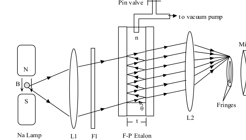
Figure 1

The Sodium lamp emits D1 ($\lambda =589.6nm$) and D2 ($589nm$) spectral lines and is located in a tunable uniform magnetic field. For simplicity, an optical filter F1 is assumed to only allow the D1 line to pass through. The D1 line is then collimated to the F-P etalon by the lens L1. Circular interference fringes will be present on the focal plane of the lens L2 with a focal length f=50cm. Different fringes have the different incident angle $\theta$. A microscope is used to observe the fringes. We take the reflectivity R=90% and the inner-surface spacing t=1cm.

Some physical constants: $h=6.626\times 10^{-34}$ J·s, $e=1.6\times 10^{-19}$ C, $m_e=9.1\times 10^{-31}$ kg, $\epsilon =3.0\times 10^{8}m{s}^{-1}$.

(a) (3points) The D1 line ($\lambda =589.6nm$) is collimated to the F-P etalon. For the vacuum case (n=1.0), please calculate (i) interference orders $m_i$, (ii) incidence angle ${\theta }_i$ and (iii) diameter $D_i$ for the first three ($i=1,2,3$) fringes from the center of the ring patterns on the focal plane.

(b) (3 points) As shown in Fig. 2, the width $\epsilon$ of the spectral line is defined as the full width of half maximum (FWHM) of light transmitivity T regarding the phase shift $\delta$. The resolution of the F-P etalon is defined as follows: for two wavelengths $\lambda$ and $\lambda +\Delta \lambda$, when the central phase difference $\Delta \delta$ of both spectral lines is larger than $\epsilon$, they are thought to be resolvable; then the etalon resolution is $\lambda /\Delta \lambda$ when $\Delta \delta =\epsilon$. For the vacuum case, the D1 line ($\lambda =589.6nm$), and because of the incident angle $\theta \approx 0$, take $\cos \theta \approx 1.0$, please calculate:

(i) the width $\epsilon$ of the spectral line;

(ii) the resolution $\lambda /\Delta \lambda$ of the etalon.

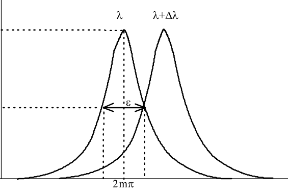
Figure 2

(c) (1 point) As shown in Fig. 1, the initial air pressure is zero. By slowly tuning the pin valve, air is gradually injected into the F-P etalon and finally the air pressure reaches the standard atmospheric pressure. On the same time, ten new fringes are observed to produce from the center of the ring patterns on the focal plane. Based on this phenomenon, calculate the refractive index of air $n_{air}$ at the standard atmospheric pressure.

(d) (2 points) Energy levels splitting of Sodium atoms occurs when they are placed in a magnetic field. This is called as the Zeeman effect. The energy shift given by $\Delta E=m_j{g}_L{\mu }_{B}B$, where the quantum number $m_j$ can be J, J-1, …, -J+1, -J. J is the total angular quantum number. $g_L$ is the Landé factor, ${\mu }_B=\frac{he}{4\pi m_e}$ is Bohr magneton, h is the Planck constant, e is the electron charge, $m_e$ is the electron mass, B is the magnetic field. As shown in Fig. 3, the D1 spectral line is emitted when Sodium atoms jump from the energy level ${}^2{P}_{1/2}$ down to ${}^2{S}_{1/2}$. We have $J=\frac{1}{2}$ for both ${}^2{P}_{1/2}$ and ${}^2{S}_{1/2}$. Therefore, in the magnetic field, each energy level will be split into two levels. We define the energy gap of two splitting levels as $\Delta E_1$ for ${}^2{P}_{1/2}$ and $\Delta E_2$ for ${}^2{S}_{1/2}$ respectively ($\Delta E_1<\Delta E_2$). As a result, the D1 line is split into 4 spectral lines (a, b, c, and d), as showed in Fig. 3. Please write down the expression of the frequency ($\nu$) of four lines a, b, c, and d.

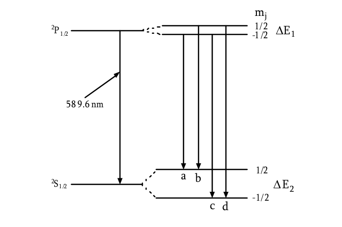
Figure 3

(e) (3 points) As shown in Fig. 4, when the magnetic field is turned on, each fringe of the D1 line will split into four sub-fringes (1, 2, 3, and 4). The diameter of the four sub-fringes near the center is measured as $D_1$, $D_2$, $D_3$, and $D_4$. Please give the expression of the splitting energy gap $\Delta E_1$ of ${}^2{P}_{1/2}$ and $\Delta E_2$ of ${}^2{S}_{1/2}$.

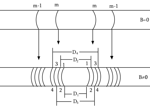
Figure 4

(f) (3 points) For the magnetic field B=0.1T, the diameter of four sub-fringes is measured as：$D_1=3.88mm$, $D_2=4.05mm$, $D_3=4.35mm$, and $D_4=4.51lmm$. Please calculate the Landé factor $g_{L1}$ of ${}^2{P}_{1/2}$ and $g_{L2}$ of ${}^2{S}_{1/2}$.

(g) (2 points) The magnetic field on the sun can be determined by measuring the Zeeman effect of the Sodium D1 line on some special regions of the sun. One observes that, in the four split lines, the wavelength difference between the shortest and longest wavelength is 0.012nm by a solar spectrograph. What is the magnetic field B in this region of the sun?

(h) (3 points) A Light-Emitting Diode (LED) source with a central wavelength $\lambda =650nm$ and spectral width $\Delta \lambda =20nm$ is normally incident ($\theta =0$) into the F-P etalon shown in Fig. 1. For the vacuum case, find (i) the number of lines in transmitted spectrum and (ii) the frequency width $\Delta \nu$ of each line?

Fonte: Testo (PDF) — p.1

Topic: Wave Optics, Modern-Quantum Physics Metodi: Interference & Diffraction Analysis, Photon Energy Relation, Small-Angle Approximation, Superposition Principle Competenze: Physical Reasoning, Experimental Data Analysis Objects: Mirror, Lens

Etalone Fabry-Perot e effetto Zeeman del sodio

La figura 1 mostra un etalon Fabry-Perot (F-P), in cui la pressione dell’aria è regolabile. L’etalon F-P è costituito da due piastre di vetro con superfici interne ad alta riflettività. Le due placche formano una cavità nella quale la luce può essere riflessa avanti e indietro. Le superfici esterne delle lastre non sono generalmente parallele alle interne e non influenzano il riflesso avanti e indietro. La densità dell’aria nell’etalon può essere controllata. La luce di una lampada a sodio viene collimata dalla lente L1 e poi passa attraverso l’etalon F-P. La trasmissibilità dell’etalon è data da $T=\frac{1}{1+F{\sin }^2(\delta /2)}$, dove

$F=\frac{4R}{(1-R{)}^2},$

$R$ è la riflettività delle superfici interne, $\delta =\frac{4\pi nt\cos \theta }{\lambda }$ è il spostamento di fase di due raggi vicini, $n$ è l’indice di rifrazione del gas, $t$ è l’intervallo delle superfici interne, $\theta$ è l’angolo di incidenza e $\lambda$ è la lunghezza d’onda di luce.

Figura 1

La lampada a sodio emette linee spettrali D1 ($\lambda =589.6nm$) e D2 ($589nm$) e si trova in un campo magnetico uniforme regolabile. Per semplificazione, si presume che un filtro ottico F1 permetta solo il passaggio della linea D1. La linea D1 viene quindi collimata all’etalon F-P dalla lente L1. I margini di interferenza circolare saranno presenti sul piano focale dell’obiettivo L2 con una lunghezza focale f=50 cm. I diversi margini hanno un’angolazione di incidenza diversa $\theta$. Un microscopio viene utilizzato per osservare i bordi. Prendiamo la riflettività R=90% e l’intervallo tra la superficie interna e l’area t=1cm.

Alcune costanti fisiche: $h=6.626\times 10^{-34}$ J·s, $e=1.6\times 10^{-19}$ C, $m_e=9.1\times 10^{-31}$ kg, $\epsilon =3.0\times 10^{8}m{s}^{-1}$.

**(a) ** **(3 punti) ** La linea D1 ($\lambda =589.6nm$) è collimata all’etalon F-P. Per il caso di vuoto (n=1.0), calcolare i) ordini di interferenza $m_i$, ii) angolo di incidenza ${\theta }_i$ e iii) diametro $D_i$ per i primi tre ($i=1,2,3$) margini dal centro dei modelli dell’anello sul piano focale.

**(b) ** **(3 punti) ** Come mostrato alla figura. 2, la larghezza $\epsilon$ della linea spettrale è definita come la larghezza completa della metà massima (FWHM) della trasmissibilità luminosa T rispetto al passaggio di fase $\delta$. La risoluzione dell’etalon F-P è definita come segue: per due lunghezze d’onda $\lambda$ e $\lambda +\Delta \lambda$, quando la differenza di fase centrale $\Delta \delta$ di entrambe le linee spettrali è maggiore di $\epsilon$, si ritiene che siano risolvibili; allora la risoluzione dell’etalon è $\lambda /\Delta \lambda$ quando $\Delta \delta =\epsilon$. Per il caso di vuoto, la linea D1 ($\lambda =589.6nm$), e a causa dell’angolo di incidenza $\theta \approx 0$, prendere $\cos \theta \approx 1.0$, calcolare:

• la larghezza $\epsilon$ della linea spettrale;

• la risoluzione $\lambda /\Delta \lambda$ dell’eccellente.

Figura 2

**(c) ** **(1 punto) ** Come mostrato alla figura. 1, la pressione iniziale dell’aria è zero. Con l’adattamento lento della valvola a pin, l’aria viene gradualmente iniettata nell’etalon F-P e infine la pressione dell’aria raggiunge la pressione atmosferica standard. Allo stesso tempo, vengono osservati dieci nuovi margini che producono da un centro degli anelli modelli sul piano focale. Sulla base di questo fenomeno calcolare l’indice di rifrazione dell’aria $n_{air}$ alla pressione atmosferica standard.

**(d) ** **(2 punti) ** Livelli energetici La divisione degli atomi di sodio si verifica quando vengono posizionati in un campo magnetico. Questo è chiamato effetto Zeeman. Il cambiamento di energia dato da $\Delta E=m_j{g}_L{\mu }_{B}B$, dove il numero quantistico $m_j$ può essere J, J-1, …, -J+1, -J. J è il numero quantistico angolare totale. $g_L$ è il fattore Landé, ${\mu }_B=\frac{he}{4\pi m_e}$ è il magnetone di Bohr, h è la costante di Planck, e è la carica di elettroni, $m_e$ è la massa di elettroni, B è il campo magnetico. Come mostrato nella figura. 3, la linea spettrale D1 viene emessa quando gli atomi di sodio saltano dal livello di energia ${}^2{P}_{1/2}$ a ${}^2{S}_{1/2}$. Abbiamo $J=\frac{1}{2}$ per entrambi ${}^2{P}_{1/2}$ e ${}^2{S}_{1/2}$. Pertanto, nel campo magnetico, ogni livello di energia sarà diviso in due livelli. Definitiamo il divario energetico di due livelli di divisione come $\Delta E_1$ per ${}^2{P}_{1/2}$ e $\Delta E_2$ per ${}^2{S}_{1/2}$ rispettivamente ($\Delta E_1<\Delta E_2$). Di conseguenza, la linea D1 è divisa in 4 linee spettrali (a, b, c e d), come mostrato in Figura. 3. Si prega di annotare l’espressione della frequenza ($\nu$) di quattro linee a, b, c e d.

Figura 3

**(e) ** **(3 punti) ** Come mostrato alla figura. 4, quando il campo magnetico è acceso, ogni margine della linea D1 si dividerà in quattro sottorini (1, 2, 3 e 4). Il diametro dei quattro sottoperiferi vicini al centro è misurato come $D_1$, $D_2$, $D_3$ e $D_4$. Indicare l’espressione del diviso energetico $\Delta E_1$ di ${}^2{P}_{1/2}$ e $\Delta E_2$ di ${}^2{S}_{1/2}$.

Figura 4

**(f) ** **(3 punti) ** Per il campo magnetico B=0,1T, il diametro di quattro sotto-margini è misurato come: $D_1=3.88mm$, $D_2=4.05mm$, $D_3=4.35mm$ e $D_4=4.51lmm$. Calcolare il fattore Landé $g_{L1}$ di ${}^2{P}_{1/2}$ e $g_{L2}$ di ${}^2{S}_{1/2}$.

Il campo magnetico sul sole può essere determinato misurando l’effetto Zeeman della linea di sodio D1 su alcune regioni speciali del sole. Si osserva che, nelle quattro linee divisi, la differenza di lunghezza d’onda tra la lunghezza d’onda più breve e più lunga è di 0,012 nm da uno spettrografo solare. Qual è il campo magnetico B in questa regione del sole?

**(h) ** **(3 punti) ** Una fonte di diodo di emissione di luce (LED) con lunghezza d’onda centrale $\lambda =650nm$ e larghezza spettrale $\Delta \lambda =20nm$ è normalmente incentrata ($\theta =0$) nell’etalon F-P riportato nella figura. 1. Per il caso del vuoto, trovare i) il numero di linee nello spettro trasmesso e ii) la larghezza di frequenza $\Delta \nu$ di ciascuna linea?

Fonte: Testo (PDF) — p.1

Topic: Wave Optics, Modern-Quantum Physics Metodi: Interference & Diffraction Analysis, Photon Energy Relation, Small-Angle Approximation, Superposition Principle Competenze: Physical Reasoning, Experimental Data Analysis Objects: Mirror, Lens