APhO 2019 — Teorica

RF reflectometry for spin readout for silicon quantum computing

Introduction

Developing the idea of quantum computing into a practical technology is one of the largest outstanding challenges in science and technology. A promising path is to manipulate individual electrons in silicon transistors by time-dependent electromagnetic fields.

In this question, we investigate the use of radio frequency (RF) reflectometry and single-electron transistors to read out the state of quantum bits in silicon-based quantum computer prototypes.

Part A and Part B discuss radio wave transmission through cables and transmission lines, part C is devoted to conditions for wave reflection, part D introduces the single-electron transistor, and parts E and F introduce and ask you to optimise the method of reflectometry.

Part A: Lumped element model of a co-axial transmission line (2.0 points)

When modelling DC or low frequency signals, one often assumes that a voltage pulse travels instantaneously throughout the circuit. This assumption is valid when the wavelength of such signals is much longer than the size of the circuit, however when working with radio frequency signals, the dynamics are more complex, and we need to account for the intrinsic capacitance and inductance of our cables in our model. We model a co-axial transmission line which acts as a waveguide as described below, ignoring the small resistance of the copper and the small conductance through the dielectric. Throughout the problem, we consider the large-wavelength limit of electromagnetic waves in the co-axial cable such that electric and magnetic fields are perpendicular to the axis of the cable everywhere (the so-called transverse electromagnetic mode).

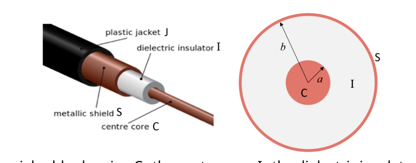Diagram of a coaxial cable showing C — the centre core, I — the dielectric insulator, S — the metallic shield and J — the plastic jacket.

Consider a co-axial cable consisting of a copper inner core of negligible resistance, negligible magnetic permeability and radius $a$, covered by an outer co-axial copper shield with inner radius $b$. A dielectric of dimensionless relative permittivity ${\epsilon }_r$ and dimensionless relative permeability ${\mu }_r$ separates the layers. When electromagnetic signals propagate through the co-axial cable, they are confined between the inner core and outer shielding.

A.1 At what speed do electromagnetic waves propagate in the co-axial cable? (0.2pt)

A.2 If there is a charge $\Delta q$ on a length $\Delta x$ of the inner core of the co-axial cable, and the outer shield is grounded, find the electric field in the region between the inner core and the shield. (0.2pt)

A.3 Find the capacitance per unit length, $C_x$, of the co-axial cable. You may wish to consider a length $\Delta x$ of the cable. (0.3pt)

A.4 Find the inductance per unit length, $L_x$, of the cable. (0.3pt)

A lumped element model of the cable is constructed by considering the inductance and capacitance of short sections of the cable. The inductance is assumed to be a property of the inner core, and the capacitance links the core with the shielding. A diagram of the lumped element model is shown below.

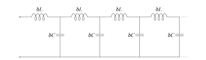Circuit diagram of lumped element model of coaxial cable.

A.5 i. Show that the impedance $Z_0$ of a semi-infinite length of cable is $Z_0=\sqrt{L_x/C_x}$. ii. Find $b/a$ if the cable has impedance $Z_0=50\Omega$ and is made using a dielectric material with ${\epsilon }_r=4.0$ and ${\mu }_r=1.0$. (1.0pt)

Part B: Hypothetical transmission line with return along a grounded plane (1.0 points)

An alternative hypothetical transmission line is shown in the diagram below. The input signal is sent through a very thin conductor of radius $a$, which is a distance $d\gg a$ from a highly conductive grounded plane. The material surrounding the conductor has dimensionless relative permittivity ${\epsilon }_r$ and dimensionless relative permeability ${\mu }_r$. The return current flows along the grounded plane.

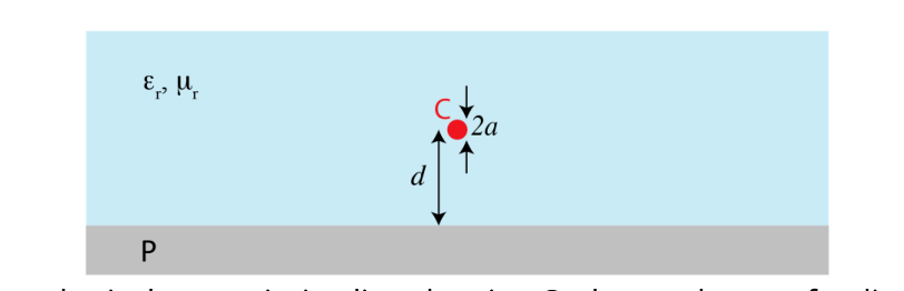Diagram of a hypothetical transmission line showing C — the conductor of radius $a$, at a distance $d\gg a$ from P — the grounded conducting plane. The conductor is embedded in a material with dimensionless relative permittivity ${\epsilon }_r$ and dimensionless relative permeability ${\mu }_r$.

B.1 Find an expression for the characteristic impedance of this hypothetical transmission line. (1.0pt)

Part C: Basics of RF reflectometry (1.2 points)

An electromagnetic wave can propagate in a transmission line in two opposite directions. For each direction of propagation, the characteristic impedance $Z_0$ can be used to relate the voltage $V_0$ and current $I_0$ amplitudes as in the Ohm’s law, $Z_0=V_0/I_0$.

Consider an interface between two transmission lines, with characteristic impedances $Z_0$ and $Z_1$. A schematic diagram of the circuit is shown below.

Circuit diagram of a transmission line of impedance $Z_0$ connected to a transmission line of impedance $Z_1$. The physical size of the interface is much smaller than the wavelength.

When a signal $V_i$ sent into the transmission line with impedance $Z_0$ reaches the interface it is partially transmitted into the second transmission line, resulting in a signal $V_t$ in that line which propagates forward. Some of the signal may also be reflected, resulting in a backward propagating signal in the initial transmission line $V_r$.

C.1 Find the reflectance of the interface $\Gamma =V_r/V_i$. (1.0pt)

C.2 State the condition(s) for the signal $V_i$ to have gained a $\pi$ phase change on reflection. (0.2pt)

Part D: The single electron transistor (3.3 points)

A single electron transistor (SET) consists of a quantum dot, which is a small isolated conductor where electrons can be localised, and of several electrodes in its vicinity. The gate electrode couples capacitatively to the quantum dot, while the two other electrodes — the source and the drain — are connected via tunnel junctions, through which electrons can tunnel due to quantum mechanics. A simplified circuit diagram for an SET is shown in the figure.

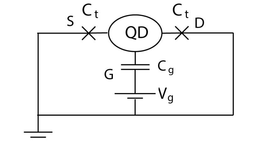Circuit diagram representation of an SET. QD is the quantum dot, S is the source, D is the drain and G is the gate.

The capacitance of the gate is $C_g$ and the capacitance of the tunnel junctions is $C_t\ll C_g$. Consider $C_g$ to be the total capacitance of the quantum dot. In this part of the problem, the source and the drain are held at zero potential, and the voltage on the gate electrode is fixed at $V_g$.

D.1 Consider a state of the SET in which the quantum dot contains $n$ electrons. i. Find the electrical potential ${\phi }_n$ on the QD. ii. Find the amount of energy $\Delta E_n$ that is necessary to bring an additional electron from the source or the drain onto the QD. (1.5pt)

If $\Delta E_n<0$ then electrons will spontaneously tunnel into the quantum dot until such a number $\mathcal{N}>n$ is reached that $\Delta E_{\mathcal{N}}\ge 0$. The equilibrium number of electrons $\mathcal{N}$ and the corresponding addition energy $\Delta E_{\mathcal{N}}$ can be controlled by choosing the appropriate voltage $V_g$.

D.2 Find an expression for the maximal possible value $E_c=\max \Delta E_{\mathcal{N}}(V_g)$ of the equilibrium addition energy that can be achieved by tuning the gate voltage of the SET. (0.5pt)

If $\Delta E_{\mathcal{N}}=0$ then tunnelling of electrons does not require extra energy and SET is in a highly conductive ON state. If $\Delta E_{\mathcal{N}}>0$, then the conductance of the SET is reduced (high-resistance OFF).

For the number of electrons on the quantum dot to remain well-defined, certain conditions need to be satisfied. Firstly, if electrons in the source or drain have thermal energies sufficient to move spontaneously onto the quantum dot, the contrast between the ON and OFF states will disappear.

D.3 Find a condition on the temperature of the electrons so that electrons cannot move onto the quantum dot by thermal excitation. (0.5pt)

Secondly, tunnelling of electrons onto or off the dot limits the lifetime of their energy states. This tunnelling can be modelled using an effective resistance of the tunnel junction with the characteristic tunnelling time equal to the characteristic time for charging or discharging the quantum dot through the junction.

D.4 i. Estimate the tunnelling time for a quantum dot in terms of capacitance $C_t$ and effective resistance $R_t$ of the tunnel junction. ii. Find a condition on the effective resistance $R_t$ so that the electrons in the quantum dot retain sufficiently well-defined energy for the ON and OFF states to remain distinct. (0.8pt)

Part E: RF reflectometry to read out SET state (1.0 points)

The state of the SET is sensitive to electrical potentials created by nearby elements of the quantum circuit (such as quantum bits), and distinguishing between ON and OFF states provides a way to read out the information produced by the quantum computer. The SET in the ON state can be modelled by a resistance $R_{\text{ON}}=100\text{k}\Omega$ while in the OFF state we can assume the SET to be a complete insulator (neglecting any capacitative connection between the source and the drain via the SET). While it is possible to determine the state of the SET by measuring the response to an input signal through the source, it is faster to do so using RF reflectometry to measure both the amplitude and phase of the reflected signal, i.e. determined the reflectance $\Gamma$.

The change in reflectance due to switching of an SET between ON and OFF states is

\Delta\Gamma = |\Gamma_{\text{ON}} - \Gamma_{\text{OFF}}|, \tag{1}

where ${\Gamma }_{\text{ON}}$ and ${\Gamma }_{\text{OFF}}$ are the reflectances in two different states.

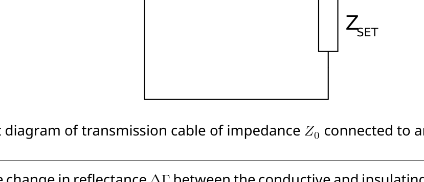Circuit diagram of transmission cable of impedance $Z_0$ connected to an SET.

E.1 Find the change in reflectance $\Delta \Gamma$ between the conductive and insulating states for a typical SET connected to a co-axial cable with impedance of $50\Omega$. (0.2pt)

In order to increase the change in reflectance, and hence the sensitivity of the RF reflectometry, the circuit is modified by inclusion of an inductor. The intrinsic capacitance due to the device geometry $C_0\approx 0.4\text{pF}$ is also taken into account. The RF reflectometry is conducted using a signal of angular frequency ${\omega }_{\text{rf}}$.

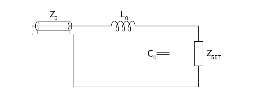Modified SET circuit.

E.2 Estimate the value of the inductance $L_0$ that can result in the change in reflection on the order of one. Calculate your estimate for $L_0$ numerically for ${\omega }_{\text{rf}}/(2\pi )=100\text{MHz}$ and compute the corresponding $\Delta \Gamma$. (0.8pt)

Part F: Charge sensing with a single lead quantum dot (1.5 points)

For a scalable quantum computing architecture, the number of wires reaching each individual quantum bit need to be minimized. A promising alternative to an SET for charge sensing in silicon quantum computing is a Single Lead Quantum Dot (SLQD). In many ways it is similar to an SET, but does not have the source and drain leads. The gate is the only electrode, through which the electron energy states of the quantum dot are controlled and also through which RF reflectometry is conducted.

Like an SET, a SLQD has an OFF in which the SLQD behaves as a total insulator. In contrast to an SET, the ON state of the SLQD is capacitive, with capacitance $C_q$. In order to maximize the difference in reflectance $\Delta \Gamma$ of the SLQD, the following circuit is constructed. The parasitic capacitance $C_0\approx 0.4\text{pF}$ is fixed by circuit geometry, but the value of $L_0$ and the operating frequency can be changed to optimize the performance. The characteristic impedance of the transmission line is $Z_0=50\Omega$.

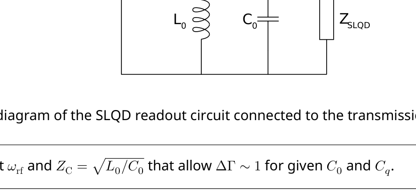Circuit diagram of the SLQD readout circuit connected to the transmission line.

F.1 Suggest ${\omega }_{\text{rf}}$ and $Z_C=\sqrt{L_0/C_0}$ that allow $\Delta \Gamma \sim 1$ for given $C_0$ and $C_q$. (1.0pt)

Optimal values of $L_0$ are relatively large and not always technically feasible. Hence, other types of circuit elements may be needed to improve sensitivity of the reflectometry readout circuit.

F.2 Assume that $L_0$ (and hence $Z_C$) is fixed. Draw a circuit diagram showing where to place an additional element in the SLQD readout circuit and specify the parameter(s) of this element such that $\Delta \Gamma \sim 1$ can still be achieved without requiring a large inductance. (0.5pt)

Fonte: Testo (PDF) — p.1

Topic: Circuits, Electromagnetism, Modern-Quantum Physics Metodi: Equivalent Circuit Reduction, Gauss’s Law, Ampère’s Law, Electric Potential Method Competenze: Mathematical Modeling, Physical Reasoning, Estimation & Approximation Objects: Wire, Capacitor, Inductor, Resistor

Refletometria RF per la lettura di spin per il calcolo quantistico del silicio

Introduzione

Sviluppare l’idea di calcolo quantistico in una tecnologia pratica è una delle più grandi sfide in sospeso nella scienza e nella tecnologia. Un percorso promettente è quello di manipolare singoli elettroni nei transistor di silicio con campi elettromagnetici dipendenti dal tempo.

In questa domanda, si indaga sull’uso della rifletometria a radio frequenza (RF) e dei transistor a singolo elettrone per leggere lo stato dei bit quantistici nei prototipi di computer quantistici a base di silicio.

La parte A e la parte B discutono la trasmissione delle onde radio attraverso cavi e linee di trasmissione, la parte C è dedicata alle condizioni per la riflessione delle onde, la parte D introduce il transistor a singolo elettrone e le parti E e F introducono e chiedono di ottimizzare il metodo di riflettimometria.

Parte A: Modello di elemento agglomerato di una linea di trasmissione coassiale (2.0 punti)

Quando si modella i segnali a corrente continua o a bassa frequenza, si assume spesso che un impulso di tensione viaggia istantaneamente attraverso il circuito. Questa ipotesi è valida quando la lunghezza d’onda di tali segnali è molto più lunga della dimensione del circuito, tuttavia quando si lavora con segnali di radio frequenza, la dinamica è più complessa e dobbiamo tenere conto della capacità intrinseca e dell’induttanza dei nostri cavi nel nostro modello. Modelliamo una linea di trasmissione coassiale che agisce come una guida d’onda come descritto di seguito, ignorando la piccola resistenza del rame e la piccola conduttività attraverso il dielettrico. Nel corso del problema, consideriamo il limite di lunghezza d’onda delle onde elettromagnetiche nel cavo coassiale in modo tale che i campi elettrici e magnetici siano perpendicolari all’asse del cavo ovunque (la cosiddetta modalità elettromagnetica trasversale).

Diagramma di un cavo coassiale che mostra C il nucleo centrale, I l’isolatore dielettrico, S lo scudo metallico e J la giacca di plastica.

Si consideri un cavo coassiale costituito da un nucleo interno di rame di resistenza trascurabile, permeabilità magnetica trascurabile e raggio $a$, coperto da uno scudo copro coassiale esterno con raggio interno $b$. Un dielettrico di relativa permitabilità dimensionaria ${\epsilon }_r$ e di relativa permeabilità dimensionaria ${\mu }_r$ separa gli strati. Quando i segnali elettromagnetici si propagano attraverso il cavo coassiale, essi sono confinati tra il nucleo interno e lo scudo esterno.

A. A che velocità si propagano le onde elettromagnetiche nel cavo coassiale? (0.2pt)

Se c’è una carica $\Delta q$ su una lunghezza $\Delta x$ del nucleo interno del cavo coassiale e lo scudo esterno è a terra, trovare il campo elettrico nella regione tra il nucleo interno e lo scudo. (0.2pt)

A.3 Trova la capacità per unità di lunghezza, $C_x$, del cavo coassiale. Potrebbe essere opportuno considerare una lunghezza $\Delta x$ del cavo. (0.3pt)

**A.4 ** Trova l’induttanza per unità di lunghezza, $L_x$, del cavo. (0.3pt)

Un modello di elemento montato del cavo viene costruito tenendo conto dell’induttanza e della capacità di sezioni brevi del cavo. Si presume che l’induttanza sia una proprietà del nucleo interno e che la capacitanza collega il nucleo al schermo. Un diagramma del modello di elementi agglomerati è mostrato di seguito.

Diagramma di circuito del modello di elemento a forma di un’insieme di cavo coassiale.

A.5 i. Indicare che l’impedenza $Z_0$ di una lunghezza semipermanente del cavo è $Z_0=\sqrt{L_x/C_x}$. ii. Trova $b/a$ se il cavo ha impedanza $Z_0=50\Omega$ e è realizzato utilizzando un materiale dielettrico con ${\epsilon }_r=4.0$ e ${\mu }_r=1.0$. (1.0pt)

Parte B: linea di trasmissione ipotetica con ritorno lungo un piano a terra (1,0 punti)

Una linea di trasmissione ipotetica alternativa è mostrata nel diagramma di seguito. Il segnale di ingresso viene inviato attraverso un conduttore molto sottile di raggio $a$, che è una distanza $d\gg a$ da un piano terraficato altamente conduttivo. Il materiale che circonda il conduttore ha una permissività relativa senza dimensioni ${\epsilon }_r$ e una permeabilità relativa senza dimensioni ${\mu }_r$. La corrente di ritorno scorre lungo il piano a terra.

Diagramma di una linea di trasmissione ipotetica che mostra C il conduttore del raggio $a$, a distanza $d\gg a$ da P il piano conduttore a terra. Il conduttore è incorporato in un materiale con permitabilità relativa senza dimensioni ${\epsilon }_r$ e permeabilità relativa senza dimensioni ${\mu }_r$.

B.1 Trova un’espressione per l’impedenza caratteristica di questa linea di trasmissione ipotetica. (1.0pt)

Parte C: Basi della rifletometria RF (1,2 punti)

Un’onda elettromagnetica può propagarsi in una linea di trasmissione in due direzioni opposte. Per ogni direzione di propagazione, l’impedenza caratteristica $Z_0$ può essere utilizzata per correlare le amplitudini di tensione $V_0$ e corrente $I_0$ come nella legge di Ohm, $Z_0=V_0/I_0$.

Si consideri un’interfaccia tra due linee di trasmissione, con impedanze caratteristiche $Z_0$ e $Z_1$. Un diagramma schematico del circuito è mostrato di seguito.

Diagramma di circuito di una linea di trasmissione di impedanza $Z_0$ collegata a una linea di trasmissione di impedanza $Z_1$. La dimensione fisica dell’interfaccia è molto più piccola della lunghezza d’onda.

Quando un segnale $V_i$ inviato nella linea di trasmissione con impedanza $Z_0$ raggiunge l’interfaccia, esso viene trasmesso in parte nella seconda linea di trasmissione, dando luogo a un segnale $V_t$ in quella linea che si propaga in avanti. Alcune parti del segnale possono anche essere riflettute, dando luogo a un segnale di propagazione all’indietro nella linea di trasmissione iniziale $V_r$.

C.1 Trova la riflessione dell’interfaccia $\Gamma =V_r/V_i$. (1.0pt)

C.2 Indicare la condizione (s) per il segnale $V_i$ di aver ottenuto un cambiamento di fase $\pi$ sulla riflessione. (0.2pt)

Parte D: Il transistor a singolo elettrone (3,3 punti)

Un singolo transistor elettronico (SET) è costituito da un punto quantistico, che è un piccolo conduttore isolato dove gli elettroni possono essere localizzati, e da diversi elettrodi nelle sue vicinanze. L’elettrodo di cancello si accoppia capacitativamente al punto quantistico, mentre gli altri due elettrodi la fonte e il drenaggio sono collegati attraverso le giunzioni di tunnel, attraverso i quali gli elettroni possono tunnelare a causa della meccanica quantistica. Il diagramma di circuito semplificato per un SET è mostrato nella figura.

Rippresentazione del diagramma di circuito di un SET. QD è il punto quantistico, S è la fonte, D è la scarico e G è la porta.

La capacità della porta è $C_g$ e la capacità delle unioni del tunnel è $C_t\ll C_g$. Considera $C_g$ la capacità totale del punto quantistico. In questa parte del problema, la fonte e il drenaggio sono tenuti a potenziale zero e la tensione sull’elettrodo di cancello è fissata a $V_g$.

D.1 Considera uno stato del SET in cui il punto quantistico contiene $n$ elettroni. i. Trova il potenziale elettrico ${\phi }_n$ sul QD. ii. Trova la quantità di energia $\Delta E_n$ necessaria per portare un elettrone aggiuntivo dalla fonte o dal drenaggio sul QD. (1.5pt)

Se $\Delta E_n<0$ allora gli elettroni si trascineranno spontaneamente nel punto quantistico fino a raggiungere un tale numero $\mathcal{N}>n$ che $\Delta E_{\mathcal{N}}\ge 0$. Il numero di equilibrio di elettroni $\mathcal{N}$ e la corrispondente energia di aggiunta $\Delta E_{\mathcal{N}}$ possono essere controllati scegliendo la voltazione appropriata $V_g$.

D.2 Trova un’espressione per il valore massimo possibile $E_c=\max \Delta E_{\mathcal{N}}(V_g)$ dell’energia di aggiunta di equilibrio che può essere ottenuta regolaendo la tensione di portale del SET. (0.5pt)

Se $\Delta E_{\mathcal{N}}=0$, il tunnelamento degli elettroni non richiede energia aggiuntiva e SET è in uno stato di ON altamente conduttivo. Se $\Delta E_{\mathcal{N}}>0$, la conduttività del SET è ridotta (OFF ad alta resistenza).

Per mantenere un numero di elettroni nel punto quantistico ben definito, occorrono soddisfare determinate condizioni. In primo luogo, se gli elettroni nella fonte o nel drenaggio hanno energie termiche sufficienti a spostarsi spontaneamente sul punto quantistico, il contrasto tra gli stati ON e OFF scomparirà.

**D.3 ** Trova una condizione sulla temperatura degli elettroni in modo che gli elettroni non possano spostarsi sul punto quantistico mediante eccitazione termica. (0.5pt)

In secondo luogo, il tunnelamento degli elettroni su o fuori il punto limita la durata degli stati energetici. Tale tunnelizzazione può essere modellata utilizzando una resistenza efficace della giunzione del tunnel con il tempo di tunnelamento caratteristico pari al tempo caratteristico per la carica o il scarico del punto quantistico attraverso la giunzione.

D.4 i. Calcolare il tempo di tunnelamento di un punto quantistico in termini di capacità $C_t$ e resistenza effettiva $R_t$ della giunzione del tunnel. ii. Trova una condizione sulla resistenza effettiva $R_t$ in modo che gli elettroni nel punto quantistico conservino energia sufficientemente ben definita per mantenere gli stati di ON e OFF distinti. (0.8pt)

Parte E: rifletometria RF per leggere lo stato SET (1,0 punti)

Lo stato del SET è sensibile ai potenziali elettrici creati da elementi vicini del circuito quantistico (come i bit quantistici), e distinguere tra stati ON e OFF fornisce un modo per leggere le informazioni prodotte dal computer quantistico. Il SET nello stato ON può essere modellato con una resistenza $R_{\text{ON}}=100\text{k}\Omega$ mentre nello stato OFF possiamo presumere che il SET sia un isolante completo (negliendone qualsiasi connessione capacitativa tra la fonte e il drenaggio tramite il SET). Mentre è possibile determinare lo stato del SET misurando la risposta a un segnale di input attraverso la sorgente, è più veloce farlo utilizzando la riflettometria a RF per misurare sia l’ampiezza che la fase del segnale riflettuto, ovvero. determinato il rifletto $\Gamma$.

La variazione della riflettività dovuta al passaggio di un SET tra stati ON e OFF è

\Delta\Gamma = |\Gamma_{\text{ON}} - \Gamma_{\text{OFF}}|, \tag{1}

dove ${\Gamma }_{\text{ON}}$ e ${\Gamma }_{\text{OFF}}$ sono le riflessioni in due stati diversi.

Diagramma di circuito di cavo di trasmissione di impedanza $Z_0$ collegato a un SET.

E.1 Trova il cambiamento di riflettività $\Delta \Gamma$ tra gli stati conduttori e isolanti per un SET tipico collegato a un cavo coassiale con impedenza $50\Omega$. (0.2pt)

Per aumentare il cambiamento di riflettività e quindi la sensibilità della rifletometria RF, il circuito viene modificato con l’inclusione di un induttore. Si tiene conto anche della capacità intrinseca derivante dalla geometria del dispositivo $C_0\approx 0.4\text{pF}$. La rifletometria RF è effettuata utilizzando un segnale di frequenza angolare ${\omega }_{\text{rf}}$.

Circuito SET modificato.

E.2 Estimare il valore dell’induttanza $L_0$ che può comportare il cambiamento della riflessione nell’ordine di uno. Calcolare numericamente la stima per $L_0$ per ${\omega }_{\text{rf}}/(2\pi )=100\text{MHz}$ e calcolare la corrispondente $\Delta \Gamma$. (0.8pt)

Parte F: Senzore di carica con un singolo punto quantistico di piombo (1,5 punti)

Per un’architettura di calcolo quantistico scalabile, il numero di fili che raggiungono ogni singolo bit quantistico deve essere ridotto al minimo. Un’alternativa promettente a un SET per la rilevazione della carica nel calcolo quantistico del silicio è un singolo punto quantistico di piombo (SLQD). In molti modi è simile a un SET, ma non ha la fonte e le condotte di scarico. Il gate è l’unico elettrodo attraverso il quale vengono controllati gli stati di energia elettronica del punto quantistico e anche attraverso il quale viene condotta la rifletometria RF.

Come un SET, un SLQD ha un OFF in cui il SLQD si comporta come isolante totale. In contrasto con un SET, lo stato ON del SLQD è capacitivo, con capacità $C_q$. Per massimizzare la differenza di riflettività $\Delta \Gamma$ del SLQD, viene costruito il seguente circuito. La capacità parassitaria $C_0\approx 0.4\text{pF}$ è fissata dalla geometria del circuito, ma il valore di $L_0$ e la frequenza di funzionamento possono essere modificati per ottimizzare le prestazioni. L’impedenza caratteristica della linea di trasmissione è $Z_0=50\Omega$.

Diagramma di circuito del circuito di lettura SLQD collegato alla linea di trasmissione.

F.1 Suggerire ${\omega }_{\text{rf}}$ e $Z_C=\sqrt{L_0/C_0}$ che consentano $\Delta \Gamma \sim 1$ per i dati $C_0$ e $C_q$. (1.0pt)

I valori ottimali di $L_0$ sono relativamente grandi e non sempre tecnicamente fattibili. Pertanto, possono essere necessari altri tipi di elementi di circuito per migliorare la sensibilità del circuito di lettura della riflettimmetria.

F.2 Supponiamo che $L_0$ (e quindi $Z_C$) sia fisso. Disegnare un diagramma di circuito che indichi dove inserire un elemento aggiuntivo nel circuito di lettura SLQD e specificare i parametri di questo elemento in modo che $\Delta \Gamma \sim 1$ possa essere ancora ottenuto senza richiedere una grande inductanza. (0.5pt)

Fonte: Testo (PDF) — p.1

Topic: Circuits, Electromagnetism, Modern-Quantum Physics Metodi: Equivalent Circuit Reduction, Gauss’s Law, Ampère’s Law, Electric Potential Method Competenze: Mathematical Modeling, Physical Reasoning, Estimation & Approximation Objects: Wire, Capacitor, Inductor, Resistor

X-ray jets from active galactic nuclei

Introduction

Active galactic nuclei (AGN) are supermassive black holes which form the centres of galaxies, and emit large amounts of energy in radiation and particle flows. One feature of many AGN are jetted outflows, which can be observed through radio emission, and sometimes also in other parts of the electromagnetic spectrum, including x-rays. These jets are large flows of plasma at relativistic speeds, over lengths of order $10^{20}\text{m}$, which is tens of thousands of light years. The x-ray emission from jets is usually dominated by synchrotron emission from relativistic electrons gyrating in the magnetic field of the jet.

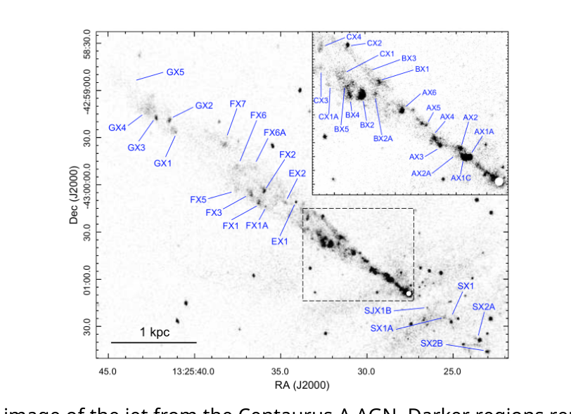Figure 1: X-ray image of the jet from the Centaurus A AGN. Darker regions represent regions of higher intensity x-rays. Brighter regions within the fainter jet are called knots. (Snios et al., 2019)

Part A: 1D fluid model of a jet

A simple model of the flow of jets assumes that the flow is steady and directed radially away from the central AGN, so approximately one dimensional, and that the plasma in the jet is in pressure equilibrium with its surroundings. There is assumed to be a constant rate per volume of mass injected into the jet from stars which lose their outer layers as they move through their life cycle.

The jet is described in terms of the coordinate representing distance from the AGN, $s$, and the opening radius $r$ of the conical jet. These distances are measured in parsecs, where $1\text{pc}=3.086\times 10^{16}\text{m}$. The speed of the jet flow is assumed to be directed radially away from the central AGN, and be a function of $s$ only. The plasma in the jet is comprised of electrons, protons, and some heavier ionised nuclei. The average energy carried by each particle in the jet, in the reference frame of the bulk flow of the jet (which we will call the jet frame), is ${ϵ}_{\text{av}}={\mu }_{pp}{c}^2+h$, where the term $h$ includes all thermal kinetic energy and potential energies in terms of the pressure $P$ and $n$ is the number density of the plasma.

As the stars, which the jet flows past, move through their life cycles they can lose part of their atmosphere. This results in a uniform rate of injection of mass per unit volume $\alpha$ into the jet, and the injected particles are assumed to be at rest relative to the AGN.

This model can be applied to the Centaurus A jet. Centaurus A is one of the nearest AGN, so it is possible to observe its jet at relatively high spatial resolution. The total power carried by the jet is estimated to be $P_j=1\times 10^{36}\text{J}\cdot {\text{s}}^{-1}$. See below for a diagram of a simple geometrical description of the Centaurus A jet, including measurements of some jet parameters. $s_1$ is the coordinate of the start of the jet, and $s_2$ the coordinate of the end of the jet. In Centaurus A the average mass per particle is ${\mu }_{pp}=0.59m_p$ and $h=\frac{13}{4}P/n$. The pressure in the plasma surrounding the jet is $P(s)=5.7\times 10^{-12}{\left(\frac{s}{s_0}\right)}^{-1.5}\text{Pa}$, where $s_0=1\text{kpc}$.

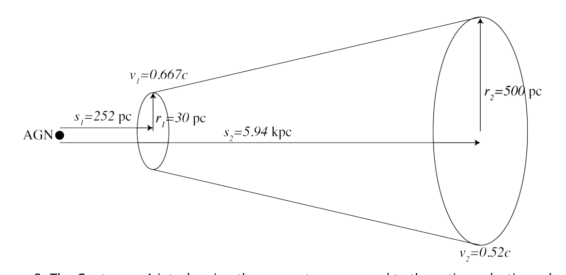Figure 2: The Centaurus A jet, showing the geometry compared to the active galactic nucleus (AGN). Labelled values: $s_1=252\text{pc}$, $r_1=30\text{pc}$, $v_1=0.667c$, $s_2=5.94\text{kpc}$, $r_2=500\text{pc}$, $v_2=0.52c$.

The jet is described by the following parameters, all of which depend on the distance $s$ from the AGN:

• the opening radius of the jet $r(s)$ in the AGN frame
• the cross sectional area of the jet $A(s)$ in the AGN frame
• the speed of the jet $v(s)$ in the AGN frame
• the lorentz gamma factor of the jet $\gamma (s)$ in the AGN frame
• the number density $n(s)$ in the frame of the jet

Any of these parameters can be used in your answers to A1–4.

A.1 Find the number density of particles, $n^{\prime }(s)$, in the frame of the AGN, in terms of the proper number density, $n(s)$ and other jet parameters. The proper number density is the number density in the frame which is locally co-moving with the jet plasma outflow, which we will call the jet frame. (0.3pt)

A.2 Find the flux of particles, $F_p(s)$, across a cross section of the jet with area $A$, at a distance $s$ from the AGN. (0.2pt)

A.3 Write a continuity relationship between the particle flux into the jet and out of the jet in terms of the jet parameters at $s_1$ and $s_2$, and $V$, the total volume of the Centaurus A jet and other required parameters. (0.5pt)

A.4 Write a relationship between the energy flux into the jet, and the energy flux out of the jet in terms of the jet speeds, cross sectional areas and proper number densities at $s_1$ and $s_2$, the volume, $V$, of the jet and any other required parameters of the Centaurus A jet. (0.6pt)

The power carried by a jet is defined to be the sum of the total bulk kinetic energy flux and the total thermal energy flux, so

P_j(s) = F_E(s) - \dot{M} c^2 \tag{1}

where $F_E(s)$ is the flux of energy through the cross section of the jet at $s$, and $\dot{M}$ is the mass flux through the jet cross section at the same distance $s$ from the AGN.

A.5 Using your answers to previous parts find $\frac{d{P}_j}{ds}$. (0.6pt)

A.6 Find numerical values for the mass fluxes ${\dot{M}}_1$, into the Centaurus A jet at $s_1$, and also ${\dot{M}}_2$, out of the Centaurus A jet at $s_2$. (0.4pt)

A.7 Find an expression for the total momentum flux, $\Pi$, into the Centaurus A jet. Also numerically evaluate this expression. (0.5pt)

A.8 Find a numerical value for the total force due to external pressure, $F_{\text{Pr}}$, on the Centaurus A jet. (0.5pt)

A.9 Write the expected relationship between $\Pi$ and $F_{\text{Pr}}$. Also, calculate the percentage difference between the model value of $\Pi$, which you found in A7, and the expected value. (0.2pt)

Part B: Gas of ultra relativistic electrons

Consider a gas of ultra relativistic electrons ($\gamma \gg 1$), with an isotropic distribution of velocities (does not depend on direction). The proper number density of particles with energies between $ϵ$ and $ϵ+dϵ$ is given by $f(ϵ)dϵ$, where $ϵ$ is the energy per particle. Consider also a wall of area $\Delta A$, which is in contact with the gas.

B.1 Write an integral expression for the total energy per volume of the electron gas. (0.2pt)

B.2 Find an expression for the total rate of change in momentum $\Delta p_z/\Delta t$ of the gas, in the z-direction which is normal to the wall, due to collisions with the wall. (0.8pt)

B.3 Derive an equation of state for an ultra relativistic electron gas, relating the pressure, volume and total internal energy. (0.6pt)

B.4 Derive a relationship between the pressure and volume of an ultra relativistic electron gas undergoing an adiabatic expansion. (0.6pt)

Part C: Synchrotron emission

In the jets from AGN, we have populations of highly energetic electrons in regions with strong magnetic fields. This creates the conditions for the emission of high fluxes of synchrotron radiation. The electrons are often so highly energetic, that they can be described as ultra relativistic with $\gamma \gg 1$.

C.1 Find an expression for $\Omega$, the angular frequency of gyration of an electron with lorentz factor $\gamma$ and travelling at an angle $\varphi$ to the magnetic field $B$. (0.7pt)

As the electron is accelerated due to the magnetic field it emits electromagnetic radiation. In a frame at which the electron is momentarily at rest, there is no preferred direction for the emission of the radiation. Half is emitted in the forward direction, and half in the backward direction. However, in the frame of the observer, for an electron moving at an ultra relativistic speed, with $\gamma \gg 1$, the radiation is concentrated in a forward cone with $\theta \lesssim 1/\gamma$ (so the total angle of cone is $2/\gamma$). As the electron is gyrating around the magnetic field, any observer will only see pulses of radiation as the forward cone sweeps through the line of sight.

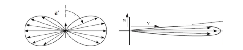Figure 3: The diagram on the left shows the distribution of power in radiation from an electron accelerating up the page in the frame at which the electron in momentarily at rest. The diagram on the right shows the distribution of power in radiation for the same electron in the observer’s frame, where most radiation is emitted in the forward cone. In the observers frame, the direction of the electron’s acceleration is shown by a vector labelled a and the direction of its velocity is shown by a vector labelled v.

C.2 Find the duration of a pulse, $\Delta t$, of synchrotron radiation observed from an electron with lorentz factor $\gamma$, travelling at an angle $\varphi$ to the magnetic field. (0.5pt)

C.3 Hence, estimate the characteristic frequency, ${\nu }_{\text{chr}}$, of the synchrotron radiation. (0.3pt)

The total synchrotron power emitted is

P_s = \frac{1}{6\pi\varepsilon_0} \left( \frac{q^4 B^2 \sin^2\phi}{m^4 c^5} \right) E^2 \tag{2}

C.4 Estimate the time, $\tau$, for an electron of energy $E$ to lose its energy through synchrotron cooling. (0.2pt)

Part D: Synchrotron emission from an AGN jet

The distribution of electron energies in a jet from an AGN is typically a power law, of the form $f(ϵ)=\kappa {ϵ}^{-p}$, where $f(ϵ)dϵ$ is the number density of particles with energies between $ϵ$ and $ϵ+dϵ$. The corresponding spectrum of synchrotron emission depends on the electron energy distribution, rather than the spectrum for an individual electron. This spectrum is

j(\nu)\,d\nu \propto B^{(1+p)/2}\,\nu^{(1-p)/2}\,d\nu. \tag{3}

Here $j(\nu )d\nu$ is the energy per unit volume emitted as photons with frequencies between $\nu$ and $\nu +d\nu$.

Observations of the Centaurus A jet, and other jets, show a knotty structure, with compact regions of brighter emission called knots. Observations of these knots at different times have shown both motion and brightness changes for some knots. Two possible mechanisms for the reductions in brightness are adiabatic expansion of the gas in the knot, and synchrotron cooling of electrons in the gas in knot.

The magnetic field in the plasma in the jets is assumed to be frozen in. Considering an arbitrary volume of plasma, the magnetic flux through the surface bounding it must remain constant, even as the volume containing the plasma changes shape and size.

D.1 For a spherical knot which expands uniformly in all directions from a volume of $V_0$ to a volume $V$, with an initial uniform magnetic field $B_0$ find the magnetic field $B$ in the expanded knot. (0.4pt)

D.2 Find $f(ϵ)$, the distribution of electron energies after adiabatic expansion of a spherical knot to a volume $V$ on the distribution of electron energy densities, given that the knot of volume $V_0$ has an initial distribution of electrons $f_0(ϵ)={\kappa }_0{ϵ}^{-p}$, where $f_0(ϵ)dϵ$ is the number density of particles with energies between $ϵ$ and $ϵ+dϵ$. (1.0pt)

D.3 How will synchrotron cooling affect the distribution of the electrons? After a time interval where electrons have been undergoing synchrotron cooling, will the distribution of electron energies as a function of $ϵ$ be steeper, shallower or leave it unchanged. Justify your answer with equations, by considering two electron energies ${ϵ}_1<{ϵ}_2$. (0.3pt)

The table below summarises some observations of knots (brighter regions) in jets from two AGN, Centaurus A (Cen A) and M87.

AGN	Time between observations	Knot	Brightness change in x-rays	Spectral changes in x-rays	Brightness changes in other bands (e.g. UV, optical)
Cen A	15 years	AX1C	−23%	No change	No data
Cen A	15 years	BX2	−15%	No change	No data
M87	5 years	HST-1	−73%	No data	No change
M87	5 years	Knot A	−12%	No data	No change

(Data from Snios et al., 2019a; 2019b.)

D.4 In the table in the answer sheet, identify the more likely cause of reduced brightness for each knot, and identify which previous part or parts support your conclusion. (0.6pt)

Fonte: Testo (PDF) — p.1

Topic: Astrophysics, Special Relativity, Electromagnetism Metodi: Relativistic Energy-Momentum, Continuity Equation, Conservation Laws, Lorentz Force Analysis Competenze: Mathematical Modeling, Estimation & Approximation, Physical Reasoning Objects: Black Hole, Electron, Photon

Gettati a raggi X provenienti da nuclei galattivi attivi

Introduzione

I nuclei galattivi attivi (AGN) sono buchi neri supermasivi che formano i centri delle galassie e emettono grandi quantità di energia nei flussi di radiazioni e particelle. Una caratteristica di molti AGN sono gli usciti di getto, che possono essere osservati attraverso l’emissione radio, e a volte anche in altre parti dello spettro elettromagnetico, compresi i raggi X. Questi getti sono grandi flussi di plasma a velocità relativistiche, su lunghezze di ordine $10^{20}\text{m}$, che è di decine di migliaia di anni luce. L’emissione di raggi X dei getti è generalmente dominata dall’emissione di sincrotroni da elettroni relativistici che girano nel campo magnetico del jet.

Figura 1: immagine a raggi X del getto dal Centaurus A AGN. Le regioni più scure rappresentano regioni di raggi X di maggiore intensità. Le regioni più luminose all’interno del jet più debole sono chiamate nodi. (Snios et al., 2019)

Parte A: modello fluido 1D di un getto

Un modello semplice del flusso di getti presuppone che il flusso sia costante e diretto radialmente lontano dal centro AGN, quindi approssimativamente a una dimensione, e che il plasma nel jet sia in equilibrio di pressione con il suo ambiente. Si presume che ci sia un tasso costante per volume di massa iniettato nel getto da stelle che perdono i loro strati esterni mentre si muovono attraverso il loro ciclo di vita.

Il getto è descritto in termini di coordinate che rappresentano la distanza dall’AGN, $s$, e il raggio di apertura $r$ del getto conico. Queste distanze sono misurate in parsecs, dove $1\text{pc}=3.086\times 10^{16}\text{m}$. La velocità del flusso di getto è presumibilmente orientata radialmente lontano dal centro AGN e è una funzione di $s$ solo. Il plasma nel getto è composto da elettroni, protoni e alcuni nuclei ionizzati più pesanti. L’energia media trasportata da ciascuna particella nel getto, nel quadro di riferimento del flusso di massa del getto (che chiameremo il jet frame), è ${ϵ}_{\text{av}}={\mu }_{pp}{c}^2+h$, dove il termine $h$ comprende tutte le energie cinetiche termali e le energie potenziali in termini di pressione $P$ e $n$ è la densità numerica del plasma.

Mentre le stelle, che il jet passa, si muovono attraverso i loro cicli di vita possono perdere parte della loro atmosfera. Ciò si traduce in un tasso uniforme di iniezione di massa per unità di volume $\alpha$ nel getto, e si presume che le particelle iniettate siano in riposo rispetto all’ AGN.

Questo modello può essere applicato al jet Centaurus A. Centaurus A è uno dei più vicini AGN, quindi è possibile osservare il suo getto a una risoluzione spaziale relativamente elevata. La potenza totale trasportata dal getto è stimata a $P_j=1\times 10^{36}\text{J}\cdot {\text{s}}^{-1}$. Si veda di seguito un diagramma di una semplice descrizione geometrica del jet Centaurus A, comprese le misurazioni di alcuni parametri del jet. $s_1$ è la coordinata della partenza del getto e $s_2$ la coordinata della fine del getto. Nel Centauro A la massa media per particella è ${\mu }_{pp}=0.59m_p$ e $h=\frac{13}{4}P/n$. La pressione plasmatica che circonda il getto è $P(s)=5.7\times 10^{-12}{\left(\frac{s}{s_0}\right)}^{-1.5}\text{Pa}$, dove $s_0=1\text{kpc}$.

Figura 2: Il getto Centaurus A, che mostra la geometria rispetto al nucleo galattico attivo (AGN). Valori etichettati: $s_1=252\text{pc}$, $r_1=30\text{pc}$, $v_1=0.667c$, $s_2=5.94\text{kpc}$, $r_2=500\text{pc}$, $v_2=0.52c$.

Il getto è descritto dai seguenti parametri, tutti dipendenti dalla distanza $s$ dall’AGN:

• il raggio di apertura del getto $r(s)$ nel quadro AGN
• la superficie trasversale del getto $A(s)$ nel telaio AGN
• la velocità del getto $v(s)$ nel quadro AGN
• il fattore gamma lorentz del getto $\gamma (s)$ nel quadro AGN
• la densità di numero $n(s)$ nel telaio del getto

Qualsiasi di questi parametri può essere utilizzato nelle risposte a A14.

**A.1 ** Trova la densità di numero delle particelle, $n^{\prime }(s)$, nel quadro dell’AGN, in termini di densità di numero appropriata, $n(s)$ e altri parametri di getto. La densità del numero corretta è la densità del numero nel telaio che si muove localmente con il flusso di plasma a getto, che chiameremo il telaio a jet. (0.3pt)

**A.2 ** Trovare il flusso di particelle, $F_p(s)$, attraverso una sezione trasversale del getto con superficie $A$, a una distanza $s$ dal GNA. (0.2pt)

A.3 Scrivere una relazione di continuità tra il flusso di particelle nel jet e fuori dal jet in termini di parametri di jet a $s_1$ e $s_2$, e $V$, il volume totale del jet Centaurus A e altri parametri richiesti. (0.5pt)

A.4 Scrivere una relazione tra il flusso di energia nel getto e il flusso di energia fuori dal jet in termini di velocità del jet, aree di sezione incrociate e densità di numero appropriato a $s_1$ e $s_2$, volume, $V$ del jet e altri parametri richiesti del jet Centaurus A. (0.6pt)

La potenza trasportata da un getto è definita come la somma del flusso totale di energia cinetica a granellamento e del flusso totale di energia termica, quindi

P_j(s) = F_E(s) - \dot{M} c^2 \tag{1}

dove $F_E(s)$ è il flusso di energia attraverso la sezione trasversale del getto a $s$, e $\dot{M}$ è il flusso di massa attraverso la sezione trasversale del getto alla stessa distanza $s$ dall’AGN.

**A.5 ** Usando le risposte alle parti precedenti trovi $\frac{d{P}_j}{ds}$. (0.6pt)

**A.6 ** Trovare valori numerici per i flussi di massa ${\dot{M}}_1$, nel getto di Centaurus A a $s_1$, e anche ${\dot{M}}_2$, fuori dal getto di Centaurus A a $s_2$. (0.4pt)

**A.7 ** Trova un’espressione per il flusso di impulso totale, $\Pi$, nel getto Centaurus A. Valutare numericamente anche questa espressione. (0.5pt)

A.8 Trova un valore numerico per la forza totale dovuta alla pressione esterna, $F_{\text{Pr}}$, sul getto Centaurus A. (0.5pt)

A.9 Scrivere la relazione attesa tra $\Pi$ e $F_{\text{Pr}}$. Calcolare inoltre la differenza percentuale tra il valore del modello di $\Pi$, che si trova in A7, e il valore atteso. (0.2pt)

Parte B: Gas di elettroni ultra relativistici

Considera un gas di elettroni ultra relativistici ($\gamma \gg 1$), con una distribuzione isotròpica delle velocità (non dipende dalla direzione). La densità di numero appropriata delle particelle con energie tra $ϵ$ e $ϵ+dϵ$ è data da $f(ϵ)dϵ$, dove $ϵ$ è l’energia per particella. Si consideri anche un muro di superficie $\Delta A$, che è in contatto con il gas.

**B.1 ** Scrivere un’espressione integrale per l’energia totale per volume del gas elettronico. (0.2pt)

B.2 Trovare un’espressione per il tasso totale di variazione del momento $\Delta p_z/\Delta t$ del gas, nella direzione z normale per la parete, a causa di collisioni con la parete. (0.8pt)

**B.3 ** Derivare un’equazione di stato per un gas elettronica ultra relativista, che relaziona la pressione, il volume e l’energia interna totale. (0.6pt)

**B.4 ** Derivare una relazione tra la pressione e il volume di un gas elettronico ultra relativistico che subisce un’espansione adiabatica. (0.6pt)

Parte C: Emissioni di sincrotroni

Nei getti di AGN, abbiamo popolazioni di elettroni altamente energetici in regioni con forti campi magnetici. Ciò crea le condizioni per l’emissione di flussi elevati di radiazioni sincrotroniche. Gli elettroni sono spesso così altamente energetici, che possono essere descritti come ultra relativistici con $\gamma \gg 1$.

C.1 Trova un’espressione per $\Omega$, la frequenza angolare di rotazione di un elettrone con fattore lorentz $\gamma$ e che viaggia ad un angolo $\varphi$ verso il campo magnetico $B$. (0.7pt)

Quando l’elettrone viene accelerato a causa del campo magnetico emette radiazioni elettromagnetiche. In un quadro in cui l’elettrone è momentaneamente a riposo, non esiste una direzione preferita per l’emissione della radiazione. La metà viene emessa in direzione anteriore e la metà in direzione anteriore. Tuttavia, nel quadro dell’osservatore, per un elettrone che si muove a velocità ultra relativistica, con $\gamma \gg 1$, la radiazione è concentrata in un cono anteriore con $\theta \lesssim 1/\gamma$ (così l’angolo totale del cono è $2/\gamma$). Mentre l’elettrone gira intorno al campo magnetico, qualsiasi osservatore vedrà solo impulsi di radiazioni mentre il cono anteriore spazza attraverso la linea di visione.

Figure 3: The diagram on the left shows the distribution of power in radiation from an electron accelerating up the page in the frame at which the electron in momentarily at rest. Il diagramma a destra mostra la distribuzione della potenza di radiazione per lo stesso elettrone nel quadro dell’osservatore, dove la maggior parte delle radiazioni viene emessa nel cono anteriore. Nel quadro degli osservatori, la direzione dell’accelerazione dell’elettrone è indicata da un vettore etichettato a e la direzione della sua velocità è indicata da un vettore etichettato v.

**C.2 ** Trova la durata di un impulso, $\Delta t$, di radiazione sincrotronico osservato da un elettrone con fattore lorentz $\gamma$, viaggiando ad un angolo $\varphi$ verso il campo magnetico. (0.5pt)

**C.3 ** Quindi, stima la frequenza caratteristica, ${\nu }_{\text{chr}}$, della radiazione sincrotronico. (0.3pt)

La potenza totale emessa dal sincrotron è

P_s = \frac{1}{6\pi\varepsilon_0} \left( \frac{q^4 B^2 \sin^2\phi}{m^4 c^5} \right) E^2 \tag{2}

**C.4 ** Estimare il tempo, $\tau$, per un elettrone di energia $E$ per perdere la sua energia attraverso il raffreddamento a sincrotrone. (0.2pt)

Parte D: Emissioni di sincrotroni da un getto AGN

La distribuzione delle energie elettroniche in uno scarico da un AGN è tipicamente una legge di potenza, della forma $f(ϵ)=\kappa {ϵ}^{-p}$, dove $f(ϵ)dϵ$ è la densità di numero di particelle con energie tra $ϵ$ e $ϵ+dϵ$. Lo spettro corrispondente di emissioni di sincrotroni dipende dalla distribuzione dell’energia degli elettroni, piuttosto che dallo spettro di un singolo elettrone. Questo spettro è

j(\nu)\,d\nu \propto B^{(1+p)/2}\,\nu^{(1-p)/2}\,d\nu. \tag{3}

Qui $j(\nu )d\nu$ è l’energia per unità di volume emessa come fotoni con frequenze tra $\nu$ e $\nu +d\nu$.

Le osservazioni del jet Centaurus A e di altri jet mostrano una struttura nodosa, con regioni compatte di emissioni più luminose chiamate nodi. Le osservazioni di questi nodi in tempi diversi hanno mostrato sia il movimento che i cambiamenti di luminosità per alcuni nodi. Due possibili meccanismi per la riduzione della luminosità sono l’espansione adiabatica del gas nel nodo e il raffreddamento sincrotronico degli elettroni nel gas nel nodo.

Si presume che il campo magnetico del plasma dei getti sia congelato. Considerando un volume arbitrario di plasma, il flusso magnetico attraverso la superficie che lo limita deve rimanere costante, anche se il volume contenente il plasma cambia forma e dimensione.

D.1 Per un nodo sferico che si espandono uniformemente in tutte le direzioni da un volume di $V_0$ a un volume di $V$, con un campo magnetico iniziale uniforme $B_0$, si trova il campo magnetico $B$ nel nodo espandito. (0.4pt)

D.2 Trova $f(ϵ)$, la distribuzione delle energie elettroniche dopo l’espansione adiabatica di un nodo sferico a un volume $V$ sulla distribuzione delle densità di energia elettronica, dato che il nodo di volume $V_0$ ha una distribuzione iniziale di elettroni $f_0(ϵ)={\kappa }_0{ϵ}^{-p}$, dove $f_0(ϵ)dϵ$ è la densità numerica di particelle con energie tra $ϵ$ e $ϵ+dϵ$. (1.0pt)

D.3 How will synchrotron cooling affect the distribution of the electrons? Dopo un intervallo di tempo in cui gli elettroni sono stati sottoposti a raffreddamento a sincrotron, la distribuzione delle energie elettroniche in funzione di $ϵ$ sarà più ripida, più bassa o non cambierà. Giustificare la risposta con le equazioni, considerando due energie elettroniche ${ϵ}_1<{ϵ}_2$. (0.3pt)

La tabella seguente riassume alcune osservazioni di nodi (regioni più luminose) nei getti di due AGN, Centaurus A (Cen A) e M87.

AgN # Tempo tra le osservazioni # Nodo # Cambiamento di luminosità nei raggi X # Cambiamenti spettrali nei raggi X # Cambiamenti di luminosità in altre bande (ad esempio UV, ottica)

|---|---|---|---|---|---| ♬ CEN A ♬ 15 anni ♬ AX1C ♬ -23% Nessun cambiamento ♬ Nessun dato ♬ CEN A 15 anni BX2 -15% Nessun cambiamento Nessun dato ♬ M87 ♬ 5 anni HST-1 ♬ -73% ♬ Nessun dato ♬ Nessun cambiamento ♬ ♬ M87 ♬ 5 anni ♬ Nodo A ♬ -12% ♬ Nessun dato ♬ Nessun cambiamento ♬

*(Dati di Snios et al., 2019a; 2019b.) *

**D.4 ** Nella tabella della scheda delle risposte, identificare la causa più probabile di riduzione della luminosità per ogni nodo e identificare quale parte o parti precedenti supportano la tua conclusione. (0.6pt)

Fonte: Testo (PDF) — p.1

Topic: Astrophysics, Special Relativity, Electromagnetism Metodi: Relativistic Energy-Momentum, Continuity Equation, Conservation Laws, Lorentz Force Analysis Competenze: Mathematical Modeling, Estimation & Approximation, Physical Reasoning Objects: Black Hole, Electron, Photon

Tippe top

Part A (10.0 points)

A Tippe top is a special kind of top that can spontaneously invert once it has been set spinning. One can model a Tippe top as a sphere of radius $R$ that is truncated, with a stem added. It has rotational symmetry about an axis through the stem, which is at angle $\theta$ from the vertical. As shown in Figure 1(a), its centre of mass $C$ is offset from its geometric centre $O$ by $\alpha R$ along its symmetry axis. The Tippe top makes contact with the surface it rests on at point $A$; we assume this surface is planar, and refer to it as the floor. Given certain geometrical constraints and if spun fast enough initially, the Tippe top will tip so that the stem points increasingly downwards, until it starts to spin on in its stem, and eventually comes to a stop.

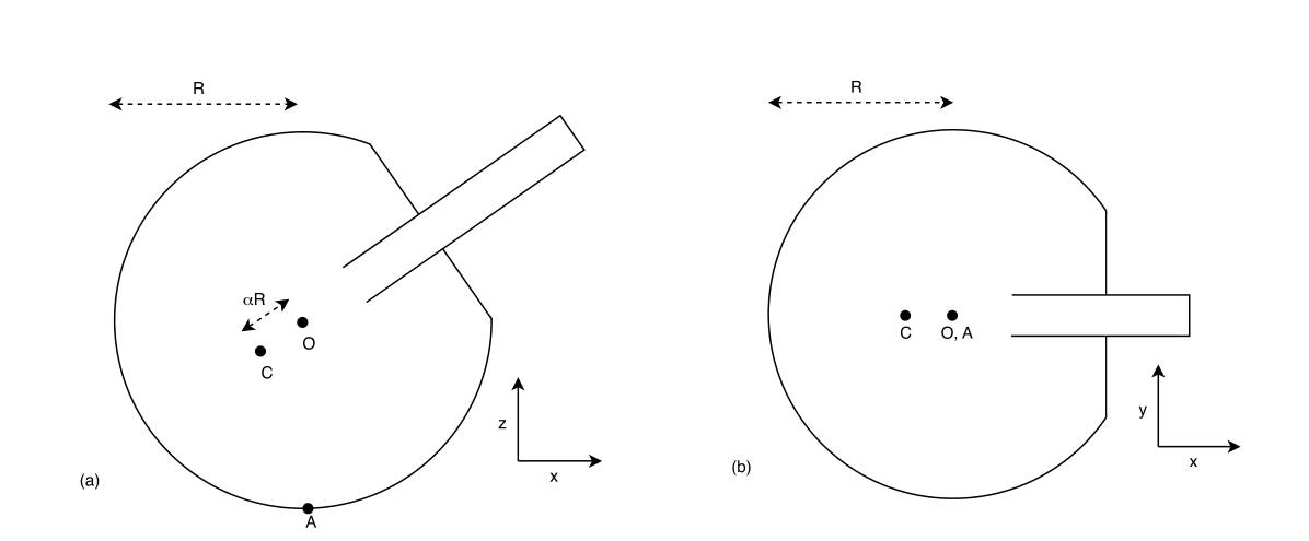Figure 1. Views of the Tippe top (a) from the side and (b) from above.

Let $xyz$ be the rotating reference frame defined such that $\hat{z}$ is stationary and upwards, and the top’s symmetry axis is within the $xz$-plane. Two views of the Tippe top are shown in Figure 1: from the side, and from above. As shown in Figure 1(b), the top’s symmetry axis is aligned with the $x$-axis when viewed from above.

Figure 2 shows the top’s motion at several phases after it is started spinning:

• A. phase I: immediately after it is initially set spinning, with $\theta \sim 0$
• B. phase II: soon after, having tipped to angle $0<\theta <\frac{\pi }{2}$
• C. phase III: when the stem first touches the floor, with $\theta >\frac{\pi }{2}$
• D. phase IV: after inversion, when the top is spinning on its stem, with $\theta \sim \pi$
• E. phase V: in its final state, at rest on its stem $\theta =\pi$.

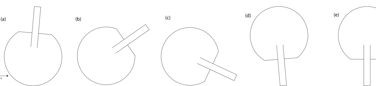Figure 2. Phases I to V of the Tippe top’s motion, shown in the $xz$-plane.

Let $XYZ$ be the inertial frame, where the surface the top is on is wholly in the $XY$-plane. The frame $xyz$ is defined as above, and reached from $XYZ$ via rotation around the $Z$ axis by $\varphi$. The transformation from the $XYZ$ frame to frame $xyz$ is shown in Figure 3(a). In particular, $\hat{z}=\hat{Z}$.

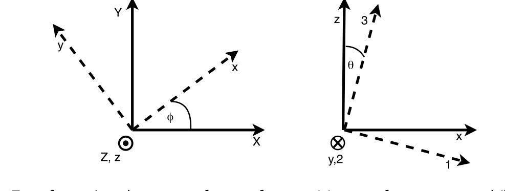Figure 3. Transformations between reference frames: (a) to $xyz$ from $XYZ$, and (b) to 123 from $xyz$.

Any rotational motion in 3-dimensional space can be described by the three Euler angles $(\theta ,\varphi ,\psi )$. The transformations between the inertial frame $XYZ$, the intermediate frame $xyz$, and the top’s frame $123$ can be understood in terms of these Euler angles.

In our description of the Tippe top’s motion, the angles $\theta$ and $\varphi$ are the standard zenith and azimuthal angles respectively, in spherical polar coordinates. In the $XYZ$ frame they are defined as follows: $\theta$ is the angle of the top’s symmetry axis from the vertical $Z$-axis, representing how far from vertical its stem is, while $\varphi$ represents the top’s angular position about the $Z$-axis, and is defined as the angle between the $XZ$-plane and the plane through points $O,A,C$ (i.e. the vertical projection of the top’s symmetry axis).

The third Euler angle $\psi$ describes the rotation of the top about its own symmetry axis, i.e. its ‘spin’, which has angular velocity $\dot{\psi }$.

The reference frame of the spinning top is defined as a new rotating frame $123$, which is reached by rotating $xyz$ by $\theta$ around $\hat{y}$: ‘tilting’ the $\hat{z}$-axis down by $\theta$ to meet the top’s symmetry axis $\hat{3}$. The transformation from the $xyz$ frame to the $123$ frame is shown in Figure 3(b). In particular, $\hat{2}=\hat{y}$.

NOTE: For a reference frame $\tilde{K}$ rotating in inertial frame $K$ with angular velocity $\omega$, the time derivatives of a vector $\mathbf{A}$ within both frames $K$ and $\tilde{K}$ are related via: \left(\frac{\partial \mathbf{A}}{\partial t}\right)_K = \left(\frac{\partial \mathbf{A}}{\partial t}\right)_{\tilde{K}} + \omega \times \mathbf{A} \tag{1}

The motion that a Tippe top undergoes is complex, involving the time evolution of the three Euler angles, as well the translational velocities (or positions) and the motion of the top’s symmetry axis. All of these parameters are coupled. To solve for the motion of a Tippe top, one would use standard tools including Newton’s laws to prepare the system of equations, then program a computer to solve them numerically via simulation.

In this question, you will perform the first part of this process, investigating the physics of the Tippe top to set up the system of equations.

Friction between the Tippe top and the surface it is moving on drives the motion of the Tippe top. Assume that the top remains in contact with the floor at point $A$, until such time as the stem contacts the floor. It is in motion at point $A$ with velocity ${\mathbf{v}}_A$ relative to the floor. The frictional coefficient ${\mu }_k$ between the top and floor is kinetic, with $|{\mathbf{F}}_f|={\mu }_{k}N$, where ${\mathbf{F}}_f=F_{f,x}\hat{x}+F_{f,y}\hat{y}$ is the frictional force, and $N$ is the magnitude of the normal force. Assume that the top is initially set spinning only, i.e. there is no translational impulse given to the top.

Let the mass of the Tippe top be $m$. Its moments of inertia are: $I_3$ about the axis of symmetry, and $I_1=I_2$ about the mutually perpendicular principal axes. Let $\mathbf{s}$ be the position vector of the centre of mass, and $\mathbf{a}=\overrightarrow{CA}$ be the vector from the centre of mass to the point of contact.

Unless otherwise specified, give your answers in the $xyz$ reference frame for full marks. All torques and angular momentum are considered about the centre of mass $C$, unless otherwise specified. You may give your answers in terms of $N$. Except for part A.8, you need only consider the top where $\theta <\frac{\pi }{2}$, and the stem is not in contact with the floor.

A.1 Find the total external force ${\mathbf{F}}_{\text{ext}}$ on the Tippe top. Draw a free body diagram of the top, projected onto each of the $xz$- and $xy$-planes. Indicate the direction of ${\mathbf{v}}_A$ in the space provided, on your diagram in the $xy$-plane. (1pt)

A.2 Find the total external torque ${\tau }_{\text{ext}}$ on the Tippe top about the centre of mass. (0.8pt)

A.3 Given the contact condition, i.e. $(\mathbf{s}+\mathbf{a})\cdot \hat{z}=0$, show that the velocity at $A$ has no component in the $z$-direction, i.e. we can write ${\mathbf{v}}_A=v_x\hat{x}+v_y\hat{y}$. (0.4pt)

A.4 Find the total angular velocity $\omega$ of the rotating top about its centre of mass $C$ in terms of the time derivatives of the Euler angles: $\dot{\theta }=\frac{d\theta }{dt},\dot{\varphi }=\frac{d\varphi }{dt},\text{and}\dot{\psi }=\frac{d\psi }{dt}.$ Use Figure 3 if this is helpful. Give your answer in the $xyz$ frame, and in the $123$ frame. (0.8pt)

A.5 Find the total energy of a spinning Tippe top, in terms of time derivatives of the Euler angles, $v_x$, and $v_y$. For partial marks, you may leave your answer in terms of $\dot{\mathbf{s}}=\frac{d\mathbf{s}}{dt}$. (1pt)

A.6 Find the rate of change of the angular momentum about the $z$-axis. (0.4pt)

A.7 Which force(s) do work against gravity? Find an expression for the instantaneous rate of change of the top’s energy — you may leave your answer in terms of ${\mathbf{v}}_A$. Identify and identify the components of the force and the torque that cause the change(s) in energy terms in A.5. (1.4pt)

A.8 Qualitatively sketch the following energy terms in the answer sheet as a function of time, over the top’s motion through the five phases I to V shown in Figure 2: the total energy $E_T$, gravitational potential energy $U_G$, translational kinetic energy $K_T$, and rotational kinetic energy $K_R$. The energy axes of your sketches are not required to be to scale. (2pt)

A.9 Show that the components of the angular momentum $\mathbf{L}$ and angular velocity $\omega$ that are perpendicular to the $\hat{3}$ direction are proportional, i.e. \mathbf{L} \times \hat{3} = k(\omega \times \hat{3}), \tag{2} and find the proportionality constant $k$. (0.5pt)

Combining your answers to A.1 and A.2 with subsequent results will give you the magnitude $N$ of the normal force, as well as a system of equations, relating the Euler angles, the components $v_x$ and $v_y$ of the velocity at $A$, the unit vector for the axis of symmetry $\hat{3}$, and their time derivatives. This system is not integrable, but instead could be solved numerically.

Integrals of motion are quantities which remain constant, and can reduce the dimensionality of the system (i.e. number of simultaneous equations to solve, whether analytically or numerically). Typically quantities such as energy, momentum, and angular momentum are conserved in closed systems, and significantly simplify the problem.

A.10 As you have seen, neither the energy nor the angular momentum are conserved for a Tippe top, due to a dissipative force and external torque. However, there is a related quantity known as Jellett’s integral $\lambda$, which represents a component of the angular momentum that is conserved, i.e. some vector $\mathbf{v}$ such that $\lambda =\mathbf{L}\cdot \mathbf{v}$ is constant in time.

Use your understanding of the Tippe top and results found so far, to give an expression for such a vector $\mathbf{v}$. Show that the time derivative of $\lambda$ is zero. (1.7pt)

Fonte: Testo (PDF) — p.1

Topic: Rotational Dynamics, Newtonian Mechanics Metodi: Torque & Angular Momentum Analysis, Free-Body Diagram, Conservation Laws, Vector Decomposition Competenze: Diagrammatic Reasoning, Mathematical Modeling, Physical Reasoning Objects: Spinning Top, Sphere

Tip top

Parte A (10,0 punti)

Una tippe top è un tipo speciale di top che può invertirsi spontaneamente una volta che è stato impostato a girare. Si può modellare un tippe top come una sfera di raggio $R$ che è troncata, con un stem aggiunto. Ha una simmetria di rotazione intorno ad un asse attraverso il tronco, che è all’angolo $\theta$ dalla verticale. Come mostrato alla figura 1 ((a), il suo centro di massa $C$ è compensato dal suo centro geometrico $O$ da $\alpha R$ lungo l’asse di simmetria. La punta superiore fa contatto con la superficie su cui si poggia al punto $A$; supponiamo che questa superficie sia piana e la chiamiamo pavimento. Data una certa restrizione geometrica e se girata abbastanza velocemente all’inizio, la punta superiore tipperà in modo che il tronco punta sempre più verso il basso, fino a quando non inizia a girare nel suo tronco, e alla fine si ferma.

Figura 1. Vede il top di Tippe (a) dal lato e (b) dall’alto.

Il $xyz$ deve essere il quadro di riferimento rotante definito in modo tale che $\hat{z}$ sia stazionario e verso l’alto, e l’asse di simmetria della parte superiore sia all’interno del piano $xz$. La figura 1 mostra due viste della punta superiore: da un lato e dall’altro. Come mostrato alla figura 1 ((b), l’asse di simmetria della parte superiore è allineato all’asse $x$ quando viene visto dall’alto.

La figura 2 mostra il movimento della parte superiore in diverse fasi dopo aver iniziato a girare:

• A. fase I: immediatamente dopo la fissazione iniziale di rotazione, con $\theta \sim 0$
• B. fase II: poco dopo, dopo aver inclinato l’angolo $0<\theta <\frac{\pi }{2}$
• C. fase III: quando il tronco tocca per la prima volta il pavimento, con $\theta >\frac{\pi }{2}$
• D. fase IV: dopo l’inversione, quando la parte superiore gira sul suo tronco, con $\theta \sim \pi$
• E. fase V: in stato finale, a riposo sul suo tronco $\theta =\pi$.

Figura 2. Fase I-V del movimento della punta superiore, mostrate nel piano $xz$.

Il $XYZ$ è il quadro inerziale, dove la superficie sulla quale si trova la parte superiore è interamente nel piano $XY$. Il telaio $xyz$ è definito come sopra e raggiunto da $XYZ$ attraverso la rotazione intorno all’asse $Z$ da $\varphi$. La trasformazione da $XYZ$ a $xyz$ è mostrata nella figura 3(a). In particolare, $\hat{z}=\hat{Z}$.

Figura 3. Trasformazioni tra quadri di riferimento: a) a $xyz$ da $XYZ$ e b) a 123 da $xyz$.

Qualsiasi movimento di rotazione nello spazio tridimensionale può essere descritto con i tre angoli di Euler $(\theta ,\varphi ,\psi )$. Le trasformazioni tra il telaio inerziale $XYZ$, il telaio intermedio $xyz$ e il telaio superiore $123$ possono essere comprese in termini di questi angoli di Euler.

Nella nostra descrizione del movimento della punta, gli angoli $\theta$ e $\varphi$ sono rispettivamente gli angoli zenit e azimuthal standard, in coordinate polari sferiche. Nel quadro $XYZ$ sono definiti come segue: $\theta$ è l’angolo dell’asse di simmetria della parte superiore rispetto all’asse verticale $Z$, che rappresenta la distanza dalla verticale del suo tronco, mentre $\varphi$ rappresenta la posizione angolare della parte superiore intorno all’asse $Z$, e è definito come l’angolo tra il piano $XZ$ e il piano attraverso i punti $O,A,C$ (cioè: la proiezione verticale dell’asse di simmetria della parte superiore).

Il terzo angolo di Euler $\psi$ descrive la rotazione della parte superiore intorno al suo asse di simmetria, ovvero il suo “spin”, che ha una velocità angolare $\dot{\psi }$.

Il telaio di riferimento della parte superiore di rotazione è definito come un nuovo telaio rotante $123$, che si ottiene ruotando $xyz$ da $\theta$ attorno a $\hat{y}$: “inclinando” l’asse $\hat{z}$ verso il basso di $\theta$ per raggiungere l’asse di simmetria della parte superiore $\hat{3}$. La trasformazione dal telaio $xyz$ al telaio $123$ è mostrata alla figura 3(b). In particolare, $\hat{2}=\hat{y}$.

**Nota: ** Per un quadro di riferimento $\tilde{K}$ che ruota in quadro inerziale $K$ con velocità angolare $\omega$, le derivate temporali di un vettore $\mathbf{A}$ all’interno di entrambi i quadri $K$ e $\tilde{K}$ sono correlate tramite: \left(\frac{\partial \mathbf{A}}{\partial t}\right)_K = \left(\frac{\partial \mathbf{A}}{\partial t}\right)_{\tilde{K}} + \omega \times \mathbf{A} \tag{1}

Il movimento che un top di Tippe subisce è complesso, coinvolgendo l’evoluzione temporale dei tre angoli di Euler, nonché le velocità di traslazione (o posizioni) e il movimento dell’asse di simmetria della cima. Tutti questi parametri sono accoppiati. Per risolvere il movimento di una tippe top, si utilizzerebbe strumenti standard tra cui le leggi di Newton per preparare il sistema di equazioni, quindi programmare un computer per risolverli numericamente tramite simulazione.

In questa domanda, si eseguirà la prima parte di questo processo, indagando la fisica della tippe top per impostare il sistema di equazioni.

La frizione tra la punta di punta e la superficie su cui si muove guida il movimento della punta di punta. Supponiamo che la parte superiore rimanga in contatto con il pavimento al punto $A$, fino a quando il tronco non entra in contatto con il pavimento. Si muove al punto $A$ con velocità ${\mathbf{v}}_A$ rispetto al pavimento. Il coefficiente di attrito ${\mu }_k$ tra la parte superiore e il pavimento è cinetico, con $|{\mathbf{F}}_f|={\mu }_{k}N$, dove ${\mathbf{F}}_f=F_{f,x}\hat{x}+F_{f,y}\hat{y}$ è la forza di attrito e $N$ è la magnitudine della forza normale. Supponiamo che la parte superiore sia inizialmente impostata solo a rotazione, cioè Non c’è nessun impulso traslazionale dato alla cima.

La massa della punta superiore deve essere $m$. I suoi momenti di inerzia sono: $I_3$ circa l’asse di simmetria, e $I_1=I_2$ circa gli assi principali reciprocamente perpendicolari. Il $\mathbf{s}$ deve essere il vettore di posizione del centro di massa e $\mathbf{a}=\overrightarrow{CA}$ deve essere il vettore dal centro di massa al punto di contatto.

Salvo indicazione contraria, fornire le risposte nel quadro di riferimento $xyz$ per i marchi completi. Tutti i coppi e il momento angolare sono considerati circa il centro di massa $C$, salvo diversa specifica. Le risposte possono essere fornite in termini di $N$. Con l’eccezione della parte A.8, occorre considerare solo la parte superiore dove $\theta <\frac{\pi }{2}$ e il tronco non è in contatto con il pavimento.

A.1 Trova la forza esterna totale ${\mathbf{F}}_{\text{ext}}$ sulla parte superiore del Tippe. Disegnare un diagramma di corpo libero della parte superiore, proiettato su ciascuno dei piani $xz$- e $xy$. Indicare la direzione di ${\mathbf{v}}_A$ nello spazio fornito, sul diagramma nel piano $xy$. (1pt)

A.2 Trova la coppia esterna totale ${\tau }_{\text{ext}}$ sulla punta superiore circa il centro di massa. (0.8pt)

**A.3 ** Data la condizione di contatto, cioè $(\mathbf{s}+\mathbf{a})\cdot \hat{z}=0$, mostrano che la velocità a $A$ non ha componente nella direzione $z$, cioè Possiamo scrivere ${\mathbf{v}}_A=v_x\hat{x}+v_y\hat{y}$. (0.4pt)

**A.4 ** Trova la velocità angolare totale $\omega$ della parte superiore rotante intorno al suo centro di massa $C$ in termini di derivati temporali degli angoli di Euler: $\dot{\theta }=\frac{d\theta }{dt},\dot{\varphi }=\frac{d\varphi }{dt},\text{and}\dot{\psi }=\frac{d\psi }{dt}.$ Se è utile, utilizzare la figura 3. Rispondi nel quadro $xyz$ e nel quadro $123$. (0.8pt)

**A.5 ** Trova l’energia totale di una tippe top in rotazione, in termini di derivati temporali degli angoli di Euler, $v_x$ e $v_y$. Per i segni parziali, la risposta può essere indicata in $\dot{\mathbf{s}}=\frac{d\mathbf{s}}{dt}$. (1pt)

**A.6 ** Trova il tasso di variazione del momento angolare intorno all’asse $z$. (0.4pt)

Quale forza opera contro la gravità? Trova un’espressione per il tasso di cambiamento istantaneo dell’energia della parte superiore puoi lasciare la tua risposta in termini di ${\mathbf{v}}_A$. Identificare e identificare i componenti della forza e della coppia che causano il cambiamento delle energie in termini di energia in A.5. (1.4pt)

A.8 Sfogliare qualitativamente i seguenti termini energetici nella scheda di risposta in funzione del tempo, sul movimento della parte superiore attraverso le cinque fasi I-V mostrate alla figura 2: l’energia totale $E_T$, l’energia potenziale gravitazionale $U_G$, l’energia cinetica traslazionale $K_T$ e l’energia cinetica rotazionale $K_R$. Gli assi energetici dei tuoi disegni non sono necessari per essere a scala. (2pt)

A.9 Mostra che le componenti del momento angolare $\mathbf{L}$ e della velocità angolare $\omega$ perpendicolari alla direzione $\hat{3}$ sono proporzionali, cioè \mathbf{L} \times \hat{3} = k(\omega \times \hat{3}), \tag{2} e trovare la costante di proporzionalità $k$. (0.5pt)

Combinando le risposte a A.1 e A.2 con i risultati successivi si ottiene la magnitudine $N$ della forza normale, nonché un sistema di equazioni, che si riferiscono agli angoli di Euler, alle componenti $v_x$ e $v_y$ della velocità a $A$, al vettore unitario per l’asse di simmetria $\hat{3}$ e alle loro derivate temporali. Questo sistema non è integrabile, ma potrebbe essere risolto numericamente.

Gli integrali di movimento sono quantitativi che rimangono costanti e possono ridurre la dimensionalità del sistema (cioè numero di equazioni simultanee da risolvere, sia analiticamente che numericamente). Tipicamente, quantità come energia, impulso e impulso angolare sono conservate in sistemi chiusi e semplificano significativamente il problema.

Come si è visto, né l’energia né il momento angolare sono conservati per un tippe top, a causa di una forza di dissipazione e di una coppia esterna. Tuttavia, esiste una quantità correlata nota come integrale di Jellett $\lambda$, che rappresenta una componente del momento angolare che viene conservato, ovvero un qualche vettore $\mathbf{v}$ tale che $\lambda =\mathbf{L}\cdot \mathbf{v}$ sia costante nel tempo.

Utilizzare la vostra comprensione della tip top e dei risultati trovati finora, per dare un’espressione per tale vettore $\mathbf{v}$. Indicare che la derivata temporale di $\lambda$ è zero. (1.7pt)

Fonte: Testo (PDF) — p.1

Topic: Rotational Dynamics, Newtonian Mechanics Metodi: Torque & Angular Momentum Analysis, Free-Body Diagram, Conservation Laws, Vector Decomposition Competenze: Diagrammatic Reasoning, Mathematical Modeling, Physical Reasoning Objects: Spinning Top, Sphere