APhO 2022 — Teorica

The Stern-Gerlach Experiment

The Stern-Gerlach experiment was performed in 1922 and it eventually led to the determination of the magnetic moment of the electron. In this experiment a beam of silver atoms each of mass $m=1.80\times 10^{-25}$ kg emerges from an oven kept at temperature $T=1.20\times 10^3$ K (see Figure 1). Assume that on emerging from the oven all the atoms have the same momentum along the direction of the beam ($z$-direction). Ignore gravity.

H. S. Mani (former Director, HRI, Prayagraj) and Gautam Datta (DAIICT, Gandhinagar) were the principal authors of this problem. The contributions of the Academic Committee, Academic Development Group, and the International Board are gratefully acknowledged.

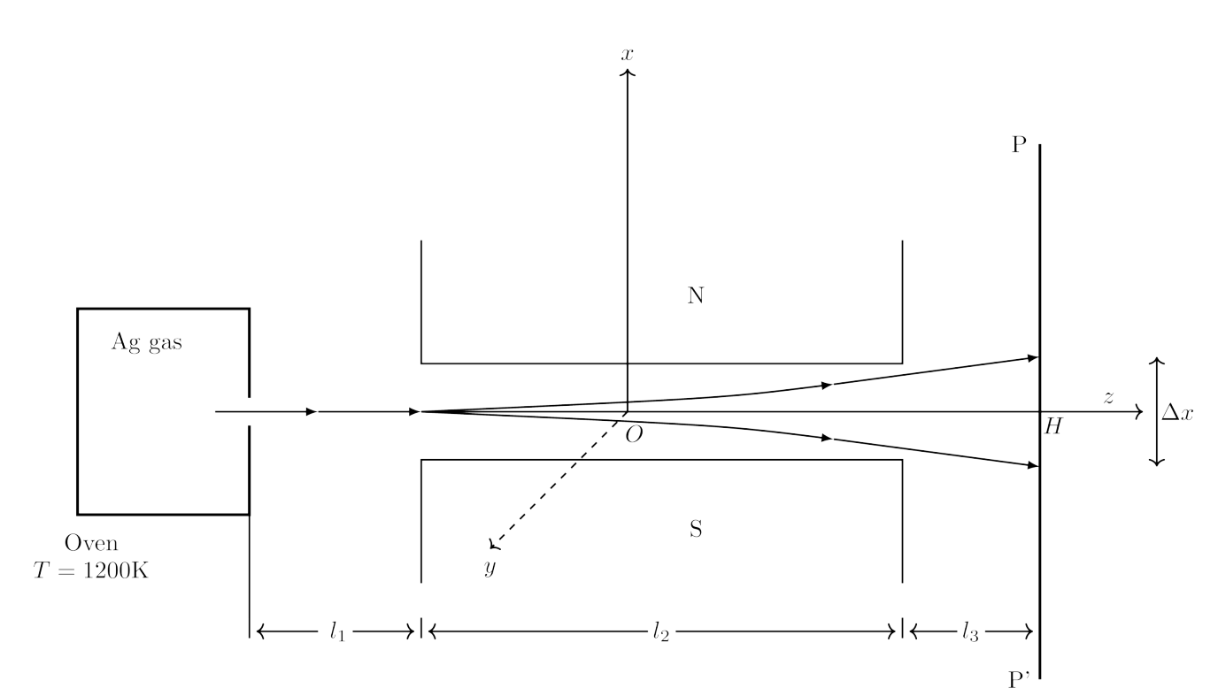Figure 1: Schematic diagram of the Stern-Gerlach setup.

A.1 (0.5pt) Speed of the Silver Atoms: The speed $v_z$ of the silver atoms emerging from the oven can be estimated to be $\sqrt{3k_{B}T/m}$ using the equipartition theorem. Calculate this value.

B.1 (2pt) The Basic Expression: After emerging from the oven the silver atoms move along the $z$-direction over a distance $l_1=0.25$ m. Next, the silver atoms pass between two magnets over a distance $l_2=0.5$ m. The magnets produce inhomogeneous magnetic field $B$ in the $x$-direction with constant gradient $dB/dx$. Assume that the silver atom has a magnetic moment pointing either in $+x$-direction or $-x$-direction, i.e. ${\vec{\mu }}_s=\pm {\mu }_s\hat{ı}$. After passing through the magnets the silver atoms pass through a further distance $l_3=0.25$ m before striking the screen $P{P}^{\prime }$. The distance between the two striking beams on the screen is $\Delta x$. Derive the expression for the splitting distance $\Delta x$ on the screen.

The Inhomogeneous Magnetic Field:

This part is concerned with the setup to create the inhomogeneous magnetic field ($dB/dx\ne 0$). It consists of a number of sub-parts. Two very long wires parallel to the $z$-axis carry currents of magnitude $I_0$ and are located at $A_1(0,-a,z)$ and $A_2(0,a,z)$ (see figure below). The direction of the current passing through $y=-a$ is $-\hat{k}$ and for the one passing through $y=a$ is $\hat{k}$. The entire system is inside a medium of high relative magnetic permeability ${\mu }_r$. We take $\mu ={\mu }_0{\mu }_r$. The wires are insulated and no current leaks into the medium.

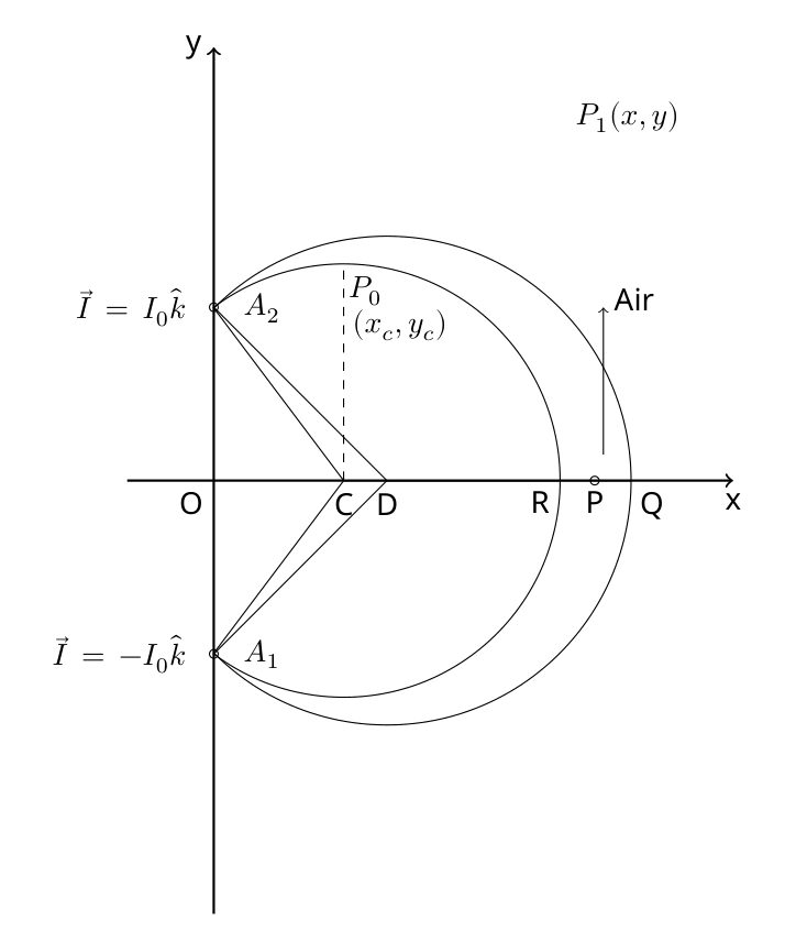Figure 2: The arrangement for the inhomogeneous magnetic field.

C.1 (1.5pt) Derive the expression for the magnetic field vector at a point $P_1(x,y,0)$ in the $x$-$y$ plane (see Fig. 2).

C.2 (0.5pt) Consider a circle with its centre $C$ on the $x$-axis $(x_c,0)$ and with radius equal to the distance $AC$ (see Figure 2). Obtain the direction of the magnetic field at circumferential points $R$ (on the $x$ axis) and at $P_0$ ($C{P}_0$ is parallel to the $y$ axis).

C.3 (0.5pt) Now a small slice of the high magnetic permeability medium between the circles with radii $AC$ and $AD$ is removed and replaced with air at very low pressure (see Fig. 2). One can show from continuity considerations that the magnetic field in this gap region is given by the same expression as if the magnetic medium were not removed. (We shall assume this and you are not required to prove this). Hence state the expression for the magnetic field at the point $(x,0)$ in the air gap region.

D.1 (0.5pt) The Force: As mentioned earlier the silver atoms are travelling in the $(x,0,z)$ plane with their velocities parallel to the $z$-axis and given by $\vec{v}=v_z\hat{k}$. Recall also that the magnetic dipole of the silver atom is ${\vec{\mu }}_s=\pm {\mu }_s\hat{ı}$. Obtain the expression for the magnitude of the force $F_x$ acting on a silver atom along the $x$-direction in terms of ${\mu }_s$, $I_0$, $a$, $\mu$ and relevant coordinates.

E.1 (2.0pt) The Magnetic Field and its Gradient: We assume that this same force $F_x$ acts over a small distance $l_2$ along the $z$ axis (Figure 1). Assume also that the silver atoms pass through the mid-point $P$ of $RQ$ (Figure 2). The following experimental values are given:

$\frac{\mu }{{\mu }_0}=10^4;a=0.60\text{ cm};OC=0.60\text{ cm};OD=0.80\text{ cm};I_0=2.00\text{ A}$

Here ${\mu }_0$ is the magnetic permeability of free space. Obtain the numerical value of the magnitudes of the magnetic field $B_P$ and its gradient $d{B}_P/dx$ at this mid-point in S.I. units.

F.1 (1.5pt) The Magnetic Moment of the Silver Atom: If $v_z=500$ m·s${}^{-1}$ and magnetic field is calculated as above, the Stern-Gerlach experiment yields a split of $\Delta x=0.20$ cm. Obtain the value of the magnetic moment of the silver atom ${\mu }_s$ in S.I. units.

G.1 (0.5pt) The spread of the line: The silver atoms may not all have the same speed. Let there be a spread of 20 % in the beam speed. What would be the consequent spread of the dot $\delta x$ on the screen?

H.1 (0.5pt) The error in the magnetic moment: What is the consequent error bar on the evaluation of the magnetic moment $\delta {\mu }_s$?

Fonte: Testo (PDF) — p.1

Topic: Magnetism, Electromagnetism, Kinetic Theory Metodi: Biot-Savart Law, Lorentz Force Analysis, Error Propagation, Kinetic Theory of Gases Competenze: Physical Reasoning, Error Propagation, Mathematical Modeling Objects: Particle Beam, Magnet, Wire

The Stern-Gerlach Experiment

L’esperimento di Stern-Gerlach fu eseguito nel 1922 e alla fine portò alla determinazione del momento magnetico dell’elettrone. In questo esperimento, un raggio di atomi d’argento di massa $m=1.80\times 10^{-25}$ kg emerge da un forno tenuto a temperatura $T=1.20\times 10^3$ K (vedi figura 1). Supponiamo che, quando escono dal forno, tutti gli atomi abbiano lo stesso impulso lungo la direzione del fascio (direzione $z$). Ignora la gravità.

H. S. Mani (ex direttore dell’HRI, Prayagraj) e Gautam Datta (DAIICT, Gandhinagar) sono stati i principali autori di questo problema. I contributi del Comitato accademico, del gruppo di sviluppo accademico e del Consiglio internazionale sono riconosciuti con gratitudine.

Figura 1: Schema di schema dell’impostazione Stern-Gerlach.

A.1 (0.5pt) **Velocità degli Atomi d’Argento: ** La velocità $v_z$ degli atomi d’Argento che emergono dal forno può essere stimata a $\sqrt{3k_{B}T/m}$ utilizzando il teorema di equipartition. Calcola questo valore.

**B.1 ** (2pt) **L’espressione di base: ** Dopo essere usciti dal forno gli atomi d’argento si muovono lungo la direzione $z$ su una distanza $l_1=0.25$ m. Successivamente, gli atomi d’argento passano tra due magneti per una distanza $l_2=0.5$ m. I magneti producono un campo magnetico $B$ in omogeneo direzione $x$ con gradiente costante $dB/dx$. Supponiamo che l’atomo d’argento abbia un momento magnetico che punta in direzione $+x$ o $-x$, ovvero ${\vec{\mu }}_s=\pm {\mu }_s\hat{ı}$. Dopo aver attraversato i magneti, gli atomi d’argento attraversano una distanza ulteriore $l_3=0.25$ m prima di colpire lo schermo $P{P}^{\prime }$. La distanza tra i due fasci colpiscanti sullo schermo è $\Delta x$. Derivare l’espressione per la distanza di divisione $\Delta x$ sullo schermo.

**Il campo magnetico inomogeneo: **

Questa parte riguarda la configurazione per creare il campo magnetico inomogeneo ($dB/dx\ne 0$). Esso è costituito da un certo numero di sottoparti. Due fili molto lunghi paralleli all’asse $z$ trasportano correnti di magnitudo $I_0$ e si trovano a $A_1(0,-a,z)$ e $A_2(0,a,z)$ (vedere figura seguente). La direzione della corrente che passa attraverso $y=-a$ è $-\hat{k}$ e per quella che passa attraverso $y=a$ è $\hat{k}$. L’intero sistema è all’interno di un mezzo ad alta permeabilità magnetica relativa ${\mu }_r$. Prendiamo $\mu ={\mu }_0{\mu }_r$. I fili sono isolati e non c’è alcuna fuga di corrente nel mezzo.

Figura 2: Disposizioni per il campo magnetico inomogeneo.

C.1 (1.5pt) Derivare l’espressione per il vettore del campo magnetico in un punto $P_1(x,y,0)$ nel piano $x$-$y$ (vedi figura 1. 2).

C.2 (0.5pt) Considera un cerchio con il suo centro $C$ sull’asse $x$ $(x_c,0)$ e con raggio uguale alla distanza $AC$ (vedi figura 2). Ottenere la direzione del campo magnetico nei punti circonferenziali $R$ (sulla spina $x$) e a $P_0$ ($C{P}_0$ è parallelo all’asse $y$).

C.3 (0.5pt) Now a small slice of the high magnetic permeability medium between the circles with radii $AC$ and $AD$ is removed and replaced with air at very low pressure (see Fig. 2). Si può dimostrare dalle considerazioni di continuità che il campo magnetico in questa regione di gap è dato dalla stessa espressione come se il mezzo magnetico non fosse stato rimosso. (Sappiamo che è vero e non è necessario che lo proviate). Indicare quindi l’espressione del campo magnetico al punto $(x,0)$ nella regione di spazio aereo.

D.1 (0.5pt) La Forza: Come accennato in precedenza gli atomi d’argento viaggiano nel piano $(x,0,z)$ con le loro velocità parallele all’asse $z$ e dati da $\vec{v}=v_z\hat{k}$. Ricordiamo anche che il dipolo magnetico dell’atomo d’argento è ${\vec{\mu }}_s=\pm {\mu }_s\hat{ı}$. Ottenere l’espressione per la grandezza della forza $F_x$ che agisce su un atomo d’argento lungo la direzione $x$ in termini di ${\mu }_s$, $I_0$, $a$, $\mu$ e coordinate pertinenti.

**E.1 ** (2.0pt) **Il campo magnetico e il suo gradiente: ** Supponiamo che questa stessa forza $F_x$ agisca su una piccola distanza $l_2$ lungo l’asse $z$ (Figura 1). Supponiamo anche che gli atomi d’argento passino attraverso il punto medio $P$ di $RQ$ (figura 2). I seguenti valori sperimentali sono dati:

$\frac{\mu }{{\mu }_0}=10^4;a=0.60\text{ cm};OC=0.60\text{ cm};OD=0.80\text{ cm};I_0=2.00\text{ A}$

Qui ${\mu }_0$ è la permeabilità magnetica dello spazio libero. Ottenere il valore numerico delle magnitudini del campo magnetico $B_P$ e del suo gradiente $d{B}_P/dx$ a questo punto medio di S.I. Unita’.

F.1 (1.5pt) Il momento magnetico dell’atomo d’argento: Se $v_z=500$ m·s${}^{-1}$ e il campo magnetico sono calcolati come sopra, l’esperimento di Stern-Gerlach produce una divisione di $\Delta x=0.20$ cm. Ottenere il valore del momento magnetico dell’atomo d’argento ${\mu }_s$ in S.I. Unita’.

**G.1 ** (0.5pt) **La diffusione della linea: ** Gli atomi d’argento potrebbero non avere tutti la stessa velocità. Si deve avere una diffusione del 20% nella velocità del fascio. Qual è la conseguente diffusione del punto $\delta x$ sullo schermo?

H.1 (0.5pt) L’errore nel momento magnetico: Qual è la conseguente barra di errore nella valutazione del momento magnetico $\delta {\mu }_s$?

Fonte: Testo (PDF) — p.1

Topic: Magnetism, Electromagnetism, Kinetic Theory Metodi: Biot-Savart Law, Lorentz Force Analysis, Error Propagation, Kinetic Theory of Gases Competenze: Physical Reasoning, Error Propagation, Mathematical Modeling Objects: Particle Beam, Magnet, Wire

A Mechanical Model for Phase Transitions

A ring of radius $R$ has a bead of negligible size and mass $m$ threaded on it. The ring is set rotating about its vertical diameter with angular velocity $\omega$ as shown in Fig. 1. Alongside this, there is an opposing force on the bead, $F_f$, which is proportional to the normal reaction $N$, and is given by $F_f=fkN$ where $f$ is $1$ or $-1$. You are advised to employ polar coordinates $\{r,\theta \}$. As far as possible express your answers in terms of ${\omega }_c=\sqrt{g/R}$ where $g$ is the magnitude of the acceleration due to gravity.

In a phase transition the free energy, $V(\mathcal{M})$ [mechanical equivalent is potential energy] depends on the magnetization $\mathcal{M}$ as follows

$V(\mathcal{M})=a(T){\mathcal{M}}^2+b(T){\mathcal{M}}^4$

where $T\to$ temperature, $b(T)>0$ and $a(T)$ changes sign with temperature. We attempt to understand the phenomenon of phase transition using the above mentioned model.

Note 1: For circular motion of radius $R$, the velocity in polar coordinates is $\dot{\vec{r}}=R\dot{\theta }\hat{\theta }$ and the acceleration is $\ddot{\vec{r}}=-R{\dot{\theta }}^2\hat{r}+R\ddot{\theta }\hat{\theta }$. Here $\hat{r}$ and $\hat{\theta }$ are unit vectors in the radial and the tangential directions respectively.

Note 2: The direction of the opposing force say ${\vec{F}}_f$ will be denoted by $f$. Here $f=+1$ if the bead is moving in the counter-clockwise direction (of increasing $\theta$) and $f=-1$ if the bead is moving in the clockwise direction $\theta$, e.g. $f=\mathrm{sgn}(\dot{\theta })$ where $\mathrm{sgn}$ is $+1$ or $-1$ depending on whether its argument is positive or negative.

Note 3: You may find the expansions

$\sin (\theta )=\theta -{\theta }^3/6+\dots$ $\cos (\theta )=1-{\theta }^2/2+{\theta }^4/24+\dots$ $(1+x{)}^n=1+nx+\frac{n(n-1)x^2}{2}+\frac{n(n-1)(n-2)x^3}{6}+\dots$

(where $\theta$ is in radians and $|x|\ll 1$) useful for some parts of the problem.

Sitikantha Das (IIT Kharagpur) and Pramendra Ranjan Singh (Principal, Narayan College, J.P. University) were the principal authors of this problem. The contributions of the Academic Committee, Academic Development Group, and the International Board are gratefully acknowledged.

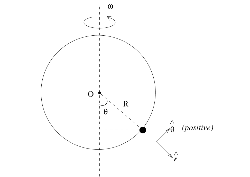Fig. 1: The bead on a rotating ring.

In what follows we shall understand the dynamics of the bead in the frame of the rotating ring and for angles in the range $-\pi /2<\theta <\pi /2$. The free body diagram of the bead is shown in Fig. 2. Neglect all forces other than the ones shown in the free body diagram.

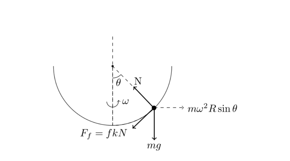Fig. 2: The free body diagram.

A.1 (0.5pt) Write down the equations of motion for the radial $F_r$ and the tangential $F_{\theta }$ components of the force on the bead. Assume $\theta$ increasing in the counter-clockwise direction.

For the following parts B.1 to B.9 assume $k=0$.

B.1 (1.0pt) State the relation between the equilibrium angle(s) ${\theta }_0$ in terms of $\{\omega ,{\omega }_c\}$.

B.2 (0.5pt) Qualitatively sketch ${\theta }_0$ ($y$-axis) as a function of $\omega /{\omega }_c$ ($x$-axis).

B.3 (0.5pt) Qualitatively sketch the magnitude of the normal reaction force on the bead as a function of $\omega /{\omega }_c$ at stable equilibrium.

B.4 (1.0pt) We define the potential energy corresponding to the tangential force $F_{\theta }$, namely

$F_{\theta }=-\frac{1}{R}\frac{d}{d\theta }V(\theta )$

with the zero of potential energy at $\theta =0$. If $V(\theta )$ is expressed as $P+Q\cos (\theta )+S{\sin }^2(\theta )$, obtain $P$, $Q$, $S$.

B.5 (1.0pt) One can expand $V(\theta )$ for small $\theta$ and express it as $V(\theta )=a(\omega ){\theta }^2+b(\omega ){\theta }^4$. Obtain the coefficients $a(\omega )$ and $b(\omega )$.

B.6 (1.0pt) Make representative plots of $V(\theta )$ versus $\theta$ for values of $\omega /{\omega }_c$ just less than $1.0$ (e.g. say $0.9$) and $\omega /{\omega }_c$ large, say $5.0$. Note that only qualitative sketches and no detailed calculations for the plots are required.

B.7 (1.0pt) Landau theory of second order phase transitions can be used to demarcate simple magnetic systems into two phases. For temperatures $T$ greater than the critical temperature $T_c$ the system is paramagnetic. For $T<T_c$ the system is ferromagnetic and the magnetization $\mathcal{M}$ is given by

$\mathcal{M}(T)={\mathcal{M}}_0(1-T/T_c{)}^{1/2}T<T_c$

Let us denote the exponent $1/2$ by $\beta$. Compare this behaviour with the bead problem discussed above. What are the analogues of $\mathcal{M}$, $T_c$, $T/T_c$ in our case? What is the equivalent value of $\beta$ in our case?

B.8 (1.0pt) Determine the angular frequency of oscillation ${\Omega }_0$ of the bead when it is disturbed from its “equilibrium” position ${\theta }_0$. Note that for small oscillations

${\Omega }_0=\frac{1}{R}\sqrt{\frac{V^{\prime \prime }({\theta }_0)}{m}}$

B.9 (1.0pt) Qualitatively sketch ${\Omega }_0$ as a function of $\omega$.

For the following parts C.1 to C.2 $k\ne 0$.

C.1 (1.0pt) Take $f=1$ and express $k=\tan \alpha$. We may express the condition for the equilibrium angle(s) ${\theta }_0$ as

${\left(\frac{\omega }{{\omega }_c}\right)}^2=\frac{\tan (x)}{\sin (y)}$

Obtain $x$ and $y$.

C.2 (0.5pt) It is given that $f=1$ and $k=0.05$. Obtain the equilibrium angles ${\theta }_0$, if any, for the following cases:

1. $\omega /{\omega }_c=0.50$
2. $\omega /{\omega }_c=0.70$

Fonte: Testo (PDF) — p.1

Topic: Newtonian Mechanics, Oscillations & Waves Metodi: Free-Body Diagram, Energy Conservation Method, Simple Harmonic Motion Analysis, Approximation & Series Expansion Competenze: Physical Reasoning, Mathematical Modeling, Diagrammatic Reasoning Objects: —

Un modello meccanico per le transizioni di fase

Un anello di raggio $R$ ha un’artigliatura di dimensioni e di massa trasversali $m$ trascinata su di esso. L’anello è impostato a rotazione intorno al suo diametro verticale con velocità angolare $\omega$ come mostrato nella figura. 1. Accanto a questo, c’è una forza opposta sulla perla, $F_f$, che è proporzionale alla reazione normale $N$, e viene data da $F_f=fkN$ dove $f$ è $1$ o $-1$. Si consiglia di utilizzare le coordinate polari $\{r,\theta \}$. Per quanto possibile, esprimere le risposte in termini di ${\omega }_c=\sqrt{g/R}$, dove $g$ è la magnitudine dell’accelerazione dovuta alla gravità.

In una transizione di fase l’energia libera $V(\mathcal{M})$ [equivalente meccanico è energia potenziale] dipende dalla magnetizzazione $\mathcal{M}$ come segue

$V(\mathcal{M})=a(T){\mathcal{M}}^2+b(T){\mathcal{M}}^4$

quando la temperatura $T\to$, $b(T)>0$ e $a(T)$ cambiano segno con la temperatura. Cerchiamo di comprendere il fenomeno della transizione di fase utilizzando il modello sopra menzionato.

**Nota 1: ** Per il movimento circolare di raggio $R$, la velocità nelle coordinate polari è $\dot{\vec{r}}=R\dot{\theta }\hat{\theta }$ e l’accelerazione è $\ddot{\vec{r}}=-R{\dot{\theta }}^2\hat{r}+R\ddot{\theta }\hat{\theta }$. Qui $\hat{r}$ e $\hat{\theta }$ sono vettori unitari rispettivamente nelle direzioni radial e tangenziale.

**Nota 2: ** La direzione della forza opposta dice ${\vec{F}}_f$ sarà indicata da $f$. Qui $f=+1$ se la perla si muove in direzione contraria al senso orario (di aumento $\theta$) e $f=-1$ se la perla si muove in senso orario $\theta$, ad esempio. $f=\mathrm{sgn}(\dot{\theta })$ in cui $\mathrm{sgn}$ è $+1$ o $-1$ a seconda che il suo argomento sia positivo o negativo.

Nota 3: ** Potete trovare le estensioni

$\sin (\theta )=\theta -{\theta }^3/6+\dots$ $\cos (\theta )=1-{\theta }^2/2+{\theta }^4/24+\dots$ $(1+x{)}^n=1+nx+\frac{n(n-1)x^2}{2}+\frac{n(n-1)(n-2)x^3}{6}+\dots$

(dove $\theta$ è in radiani e $|x|\ll 1$) utile per alcune parti del problema.

• Sitikantha Das (IIT Kharagpur) e Pramendra Ranjan Singh (Principal, Narayan College, J.P. L’Università di Lisbona (Università di Lisbona) è stata la principale autrice di questo problema. I contributi del Comitato accademico, del gruppo di sviluppo accademico e del Consiglio internazionale sono riconosciuti con gratitudine.*

Fig. 1: la perla su un anello rotante.

In quanto segue, comprenderemo la dinamica della perla nel quadro dell’anello rotante e per gli angoli nell’intervallo $-\pi /2<\theta <\pi /2$. Il diagramma del corpo libero della perla è mostrato nella figura. 2. Ignorare tutte le forze diverse da quelle mostrate nel diagramma del corpo libero.

Fig. 2: Il diagramma del corpo libero.

A.1 (0.5pt) Scrivere le equazioni di movimento per i componenti radiali $F_r$ e tangenziali $F_{\theta }$ della forza sulla perla. Supponiamo che $\theta$ si stia incrementando nella direzione contraria al senso orario.

Per le seguenti parti da B.1 a B.9 supponiamo $k=0$.

B.1 (1.0pt) Indicare la relazione tra l’angolo di equilibrio ((s) ${\theta }_0$ in termini di $\{\omega ,{\omega }_c\}$.

B.2 (0.5pt) Sceneggiare qualitativamente ${\theta }_0$ ($y$-asse) come funzione di $\omega /{\omega }_c$ ($x$-asse).

B.3 (0.5pt) Sfogliare qualitativamente la grandezza della forza di reazione normale sulla mancia come funzione di $\omega /{\omega }_c$ in equilibrio stabile.

**B.4 ** (1.0pt) Definitiamo l’energia potenziale corrispondente alla forza tangenziale $F_{\theta }$, vale a dire

$F_{\theta }=-\frac{1}{R}\frac{d}{d\theta }V(\theta )$

con il valore di energia potenziale zero a $\theta =0$. Se $V(\theta )$ è espresso come $P+Q\cos (\theta )+S{\sin }^2(\theta )$, si ottengono $P$, $Q$, $S$.

B.5 (1.0pt) Si può espandere $V(\theta )$ per $\theta$ piccolo ed esprimere come $V(\theta )=a(\omega ){\theta }^2+b(\omega ){\theta }^4$. Ottenere i coefficienti $a(\omega )$ e $b(\omega )$.

B.6 (1.0pt) Fare grafici rappresentativi di $V(\theta )$ contro $\theta$ per valori $\omega /{\omega }_c$ appena inferiori a $1.0$ (ad esempio: dire $0.9$) e $\omega /{\omega }_c$ grande, dire $5.0$. Si noti che sono necessari solo bozze qualitative e nessun calcolo dettagliato per le plot.

La teoria di Landau delle transizioni di fase di secondo ordine può essere utilizzata per demarcare i semplici sistemi magnetici in due fasi. Per temperature $T$ superiori alla temperatura critica $T_c$ il sistema è paramagnetico. Per $T<T_c$ il sistema è ferromagneto e la magnetizzazione $\mathcal{M}$ è data da

$\mathcal{M}(T)={\mathcal{M}}_0(1-T/T_c{)}^{1/2}T<T_c$

Indichiamo l’esponente $1/2$ con $\beta$. Confrontate questo comportamento con il problema della perla sopra descritto. Quali sono gli analoghi di $\mathcal{M}$, $T_c$, $T/T_c$ nel nostro caso? Qual è il valore equivalente di $\beta$ nel nostro caso?

B.8 (1.0pt) Determina la frequenza angolare di oscillazione ${\Omega }_0$ della mancia quando viene disturbata dalla sua posizione di “equilibrio” ${\theta }_0$. Si noti che per piccole oscillazioni

${\Omega }_0=\frac{1}{R}\sqrt{\frac{V^{\prime \prime }({\theta }_0)}{m}}$

B.9 (1.0pt) Sceneggiare qualitativamente ${\Omega }_0$ come funzione di $\omega$.

Per le seguenti parti da C.1 a C.2 $k\ne 0$.

**C.1 ** (1.0pt) Prendi $f=1$ e esprimi $k=\tan \alpha$. Possiamo esprimere la condizione per l’angolo di equilibrio s) ${\theta }_0$ come

${\left(\frac{\omega }{{\omega }_c}\right)}^2=\frac{\tan (x)}{\sin (y)}$

Ottenere $x$ e $y$.

**C.2 ** (0.5pt) Si dà che $f=1$ e $k=0.05$. Ottenere gli angoli di equilibrio ${\theta }_0$, se del caso, per i seguenti casi:

1. $\omega /{\omega }_c=0.50$
2. $\omega /{\omega }_c=0.70$

Fonte: Testo (PDF) — p.1

Topic: Newtonian Mechanics, Oscillations & Waves Metodi: Free-Body Diagram, Energy Conservation Method, Simple Harmonic Motion Analysis, Approximation & Series Expansion Competenze: Physical Reasoning, Mathematical Modeling, Diagrammatic Reasoning Objects: —

Maxwell, Rayleigh and Mount Everest: THE PROBLEM

Lord Rayleigh visited Darjeeling, India in 1897. On viewing Mount Everest at a distance of 170 km he was reminded of a query by James Maxwell 26 years earlier on the attenuation of light by air and the visibility of far-off peaks. Lord Rayleigh authored a famous research paper two years later in 1899 in which he investigated this problem. In the present problem we attempt to reconstruct, at least partially, a modern version of Lord Rayleigh’s line of reasoning.

Oscillation of the electron cloud: We model a typical neutral air molecule by a stationary positive charge $q$ surrounded by a spherical uniform charge cloud of mass $m$, radius $r$ and charge $-q$. The natural angular frequency of vibration of the molecule is ${\omega }_0$. Light is incident on it and the negative cloud oscillates maintaining its spherical shape with angular frequency $\omega$ as,

y = y_0 \cos(\omega t), \tag{1}

under the influence of the electric field

\vec{E}(t) = E_0 \cos(\omega t)\,\hat{y}, \tag{2}

of the light wave. Here $y$ represents the separation between the stationary positive charge and the centre of the negative charge cloud of the molecule.

Amitabh Virmani (CMI, Chennai) and A. C. Biyani (retired Govt. Nagarjuna P.G. College of Science, Raipur) were the principal authors of this problem. The contributions of the Academic Committee, Academic Development Group, and the International Board are gratefully acknowledged.

Reference: Philosophical Mag. “On the transmission of light through an atmosphere … and the origin of the blue of the sky”, Vol. 47, pg 375-384, 1899.

A.1 (0.5pt) Set up the equation for the motion for $y$. Take the contribution to the magnitude of the acceleration due to the electric field to be $E(t)q/m$.

A.2 (0.5pt) Based on the information provided above, solve the equation for $y$. Find the amplitude.

A.3 (0.5pt) Find the magnitude $p(t)$ of the dipole moment of the air molecule as a function of time for $\omega \ll {\omega }_0$.

A.4 (0.5pt) Obtain an expression for ${\omega }_0$ in terms of $q$, $m$ and $r$.

Power radiated: The sinusoidal time dependent dipole radiates electromagnetic radiation. The power radiated depends on the amplitude of the dipole moment $p_0=q{y}_0$, the permittivity of vacuum ${ϵ}_0$, the speed of light $c$, and the frequency of oscillation $\omega$.

B.1 (1pt) Use dimensional analysis to express the average power $s$ radiated in terms of these quantities.

B.2 (0.2pt) Take the proportionality constant to be $1/12\pi$. Express the answer for the power radiated $s$ in terms of $E_0$, ${\omega }_0$, $\omega$ and related quantities. Take $\omega \ll {\omega }_0$.

Attenuation of the Intensity $I(x)$: Recall that the intensity of EM waves is

\frac{1}{2} c \epsilon_0 E_0^2. \tag{3}

The intensity decreases along the path of light because the power

S = n_0 s \tag{4}

is lost per unit volume. Here $n_0$ is the number of molecules per unit volume.

C.1 (1pt) Set up the differential equation for the intensity $I(x)$ as a function of the distance $x$.

C.2 (0.5pt) Obtain the expression for the intensity $I(x)$ as a function of $x$ in terms of the characteristic length scale $L$ associated with the drop in intensity. Take the initial intensity to be $I_0$.

C.3 (0.3pt) Take $m$ to be the mass of the electron (typically only one electron constitutes the charge cloud) and take

n_0 = 2.54 \times 10^{25} \text{ m}^{-3}, \tag{5} \omega_0 = 1.25 \times 10^{16} \text{ rad·s}^{-1}, \tag{6} \omega = 3.25 \times 10^{15} \text{ rad·s}^{-1}. \tag{7}

Obtain the numerical value of $L$ in kilometers.

D.1 (2pt) Height $H^{\prime }$ of the Mountains as seen by an observer: In the figure the point $P$ denotes Darjeeling, a hill station in the eastern Himalayas at height $h=2042$ m above the sea level. The line $BS$ denotes Mt Everest which is $d=170$ km away from Darjeeling and is of height $H=8848$ m. Another peak Mount Kanchenjunga (not shown in the figure) is 75 km away from Darjeeling and is of height 8586 m. Obtain an expression and the numerical values of the vertical height $H^{\prime }$ of these mountains as seen by an observer from Darjeeling in terms of the above-mentioned quantities. Assume that the observer is unable to see below the local horizon. Draw an appropriate figure. Take the radius $R$ of the Earth to be 6378 km.

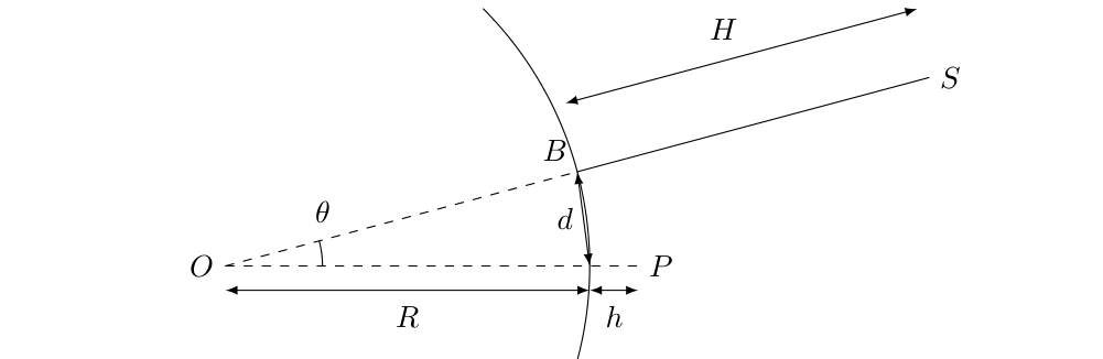Figure 1. Great circle on which lie the mountain $BS$ at height $H$ and the observer $P$ at height $h$. Note that the figure is not to scale.

E.1 (1pt) Take the intensity of Mt Kanchenjunga at Darjeeling to be the reference value. What would be the intensity of Mt Everest relative to Mt Kanchenjunga as seen from Darjeeling? In this problem we ignore the variation in the number density of air molecules with height. If the intensity is 5 % or more of the reference value the mountain is said to be visible. Will Mt Everest be visible from Darjeeling?

F.1 (1pt) Attenuation length $L_p$ due to aerosol pollution: Above, we calculated the characteristic length scale $L$ associated with the drop in intensity due to scattering with air molecules. We are now interested in the characteristic length $L_p$ associated with the drop in intensity due to scattering with aerosol particles (pollution). $L_p$ depends on the number density $n$ of particles and the cross sectional area $\pi r^2$ of the aerosol particle of radius $r$. Obtain this dependence using physical insight and dimensional analysis. Take the dimensionless constant to be $1/8$. Given mild pollution the average aerosol density at Darjeeling is ${\rho }_p=5\mu {\text{g/m}}^3$, and their average radius is 500 nanometres. What is the length $L_p$? Let the density of an individual aerosol particle be $\rho =3{\text{g/cm}}^3$. Note $1\mu \text{g}=10^{-9}$ kg and $1$ nm $=10^{-9}$ m.

G.1 (1pt) Relative intensity and Visibility of Mt. Kanchenjunga and Mt. Everest: Estimate the relative intensity of Mt Kanchenjunga and Mt Everest with the above level of pollution with respect to the reference value. Which, if any of these peaks will be visible from Darjeeling? Assume that pollution is uniform throughout the path the light travels.

Fonte: Testo (PDF) — p.1

Topic: Oscillations & Waves, Electromagnetism, Order-of-Magnitude Estimation Metodi: Dimensional Analysis, Differential Equations, Simple Harmonic Motion Analysis, Order-of-Magnitude Estimation Competenze: Physical Reasoning, Estimation & Approximation, Mathematical Modeling Objects: Atom, Electron

Maxwell, Rayleigh e il Monte Everest: IL PROBLEMA

Lord Rayleigh visitò Darjeeling, in India, nel 1897. Osservando il Monte Everest a una distanza di 170 km, si ricordò di una domanda posta da James Maxwell 26 anni prima sull’attenuazione della luce da parte dell’aria e sulla visibilità delle vette lontane. Due anni dopo, nel 1899, Lord Rayleigh scrisse un celebre articolo di ricerca in cui studiò questo problema. Nel presente problema cerchiamo di ricostruire, almeno in parte, una versione moderna del ragionamento di Lord Rayleigh.

Oscillazione della nube elettronica: Modellizziamo una tipica molecola d’aria neutra come una carica positiva fissa $q$ circondata da una nube di carica sferica e uniforme di massa $m$, raggio $r$ e carica $-q$. La frequenza angolare naturale di vibrazione della molecola è ${\omega }_0$. La luce incide su di essa e la nube negativa oscilla mantenendo la sua forma sferica con frequenza angolare $\omega$ secondo,

y = y_0 \cos(\omega t), \tag{1}

sotto l’influenza del campo elettrico

\vec{E}(t) = E_0 \cos(\omega t)\,\hat{y}, \tag{2}

dell’onda luminosa. Qui $y$ rappresenta la separazione tra la carica positiva fissa e il centro della nube di carica negativa della molecola.

Amitabh Virmani (CMI, Chennai) e A. C. Biyani (in pensione, Govt. Nagarjuna P.G. College of Science, Raipur) sono stati gli autori principali di questo problema. Si ringraziano per i loro contributi il Comitato Accademico, l’Academic Development Group e il Comitato Internazionale.

Riferimento: Philosophical Mag. “On the transmission of light through an atmosphere … and the origin of the blue of the sky”, Vol. 47, pg 375-384, 1899.

A.1 (0.5pt) Scrivi l’equazione del moto per $y$. Si assuma che il contributo al modulo dell’accelerazione dovuto al campo elettrico sia $E(t)q/m$.

A.2 (0.5pt) In base alle informazioni fornite sopra, risolvi l’equazione per $y$. Trova l’ampiezza.

A.3 (0.5pt) Trova il modulo $p(t)$ del momento di dipolo della molecola d’aria in funzione del tempo per $\omega \ll {\omega }_0$.

A.4 (0.5pt) Ricava un’espressione per ${\omega }_0$ in termini di $q$, $m$ e $r$.

Potenza irradiata: Il dipolo sinusoidale dipendente dal tempo irradia radiazione elettromagnetica. La potenza irradiata dipende dall’ampiezza del momento di dipolo $p_0=q{y}_0$, dalla permittività del vuoto ${ϵ}_0$, dalla velocità della luce $c$ e dalla frequenza di oscillazione $\omega$.

B.1 (1pt) Usa l’analisi dimensionale per esprimere la potenza media $s$ irradiata in termini di queste grandezze.

B.2 (0.2pt) Si assuma che la costante di proporzionalità sia $1/12\pi$. Esprimi il risultato per la potenza irradiata $s$ in termini di $E_0$, ${\omega }_0$, $\omega$ e grandezze correlate. Si assuma $\omega \ll {\omega }_0$.

Attenuazione dell’intensità $I(x)$: Si ricordi che l’intensità delle onde EM è

\frac{1}{2} c \epsilon_0 E_0^2. \tag{3}

L’intensità diminuisce lungo il cammino della luce perché la potenza

S = n_0 s \tag{4}

viene persa per unità di volume. Qui $n_0$ è il numero di molecole per unità di volume.

C.1 (1pt) Scrivi l’equazione differenziale per l’intensità $I(x)$ in funzione della distanza $x$.

C.2 (0.5pt) Ricava l’espressione dell’intensità $I(x)$ in funzione di $x$ in termini della lunghezza caratteristica $L$ associata al calo di intensità. Si assuma che l’intensità iniziale sia $I_0$.

C.3 (0.3pt) Si assuma che $m$ sia la massa dell’elettrone (tipicamente un solo elettrone costituisce la nube di carica) e si prenda

n_0 = 2.54 \times 10^{25} \text{ m}^{-3}, \tag{5} \omega_0 = 1.25 \times 10^{16} \text{ rad·s}^{-1}, \tag{6} \omega = 3.25 \times 10^{15} \text{ rad·s}^{-1}. \tag{7}

Ricava il valore numerico di $L$ in chilometri.

D.1 (2pt) Altezza $H^{\prime }$ delle montagne vista da un osservatore: Nella figura il punto $P$ indica Darjeeling, una stazione collinare nell’Himalaya orientale a un’altezza $h=2042$ m sul livello del mare. La linea $BS$ indica il Monte Everest, che dista $d=170$ km da Darjeeling e ha altezza $H=8848$ m. Un’altra vetta, il Monte Kanchenjunga (non mostrata nella figura), dista 75 km da Darjeeling e ha altezza 8586 m. Ricava un’espressione e i valori numerici dell’altezza verticale $H^{\prime }$ di queste montagne viste da un osservatore da Darjeeling in termini delle grandezze sopra menzionate. Si assuma che l’osservatore non sia in grado di vedere al di sotto dell’orizzonte locale. Disegna una figura appropriata. Si assuma che il raggio $R$ della Terra sia 6378 km.

Figura 1. Cerchio massimo su cui giacciono la montagna $BS$ ad altezza $H$ e l’osservatore $P$ ad altezza $h$. Si noti che la figura non è in scala.

E.1 (1pt) Si assuma come valore di riferimento l’intensità del Monte Kanchenjunga a Darjeeling. Quale sarebbe l’intensità del Monte Everest rispetto al Monte Kanchenjunga vista da Darjeeling? In questo problema trascuriamo la variazione della densità numerica di molecole d’aria con l’altezza. Se l’intensità è pari o superiore al 5 % del valore di riferimento, la montagna si dice visibile. Il Monte Everest sarà visibile da Darjeeling?

F.1 (1pt) Lunghezza di attenuazione $L_p$ dovuta all’inquinamento da aerosol: Sopra abbiamo calcolato la lunghezza caratteristica $L$ associata al calo di intensità dovuto allo scattering con le molecole d’aria. Ora ci interessa la lunghezza caratteristica $L_p$ associata al calo di intensità dovuto allo scattering con le particelle di aerosol (inquinamento). $L_p$ dipende dalla densità numerica $n$ di particelle e dalla sezione d’urto $\pi r^2$ della particella di aerosol di raggio $r$. Ricava questa dipendenza usando l’intuizione fisica e l’analisi dimensionale. Si assuma che la costante adimensionale sia $1/8$. Con un lieve inquinamento, la densità media di aerosol a Darjeeling è ${\rho }_p=5\mu {\text{g/m}}^3$ e il loro raggio medio è 500 nanometri. Quanto vale la lunghezza $L_p$? Sia la densità di una singola particella di aerosol $\rho =3{\text{g/cm}}^3$. Si noti che $1\mu \text{g}=10^{-9}$ kg e $1$ nm $=10^{-9}$ m.

G.1 (1pt) Intensità relativa e visibilità del Monte Kanchenjunga e del Monte Everest: Stima l’intensità relativa del Monte Kanchenjunga e del Monte Everest con il livello di inquinamento sopra indicato rispetto al valore di riferimento. Quale di queste vette, se ve n’è una, sarà visibile da Darjeeling? Si assuma che l’inquinamento sia uniforme lungo tutto il cammino percorso dalla luce.

Fonte: Testo (PDF) — p.1

Topic: Oscillations & Waves, Electromagnetism, Order-of-Magnitude Estimation Metodi: Dimensional Analysis, Differential Equations, Simple Harmonic Motion Analysis, Order-of-Magnitude Estimation Competenze: Physical Reasoning, Estimation & Approximation, Mathematical Modeling Objects: Atom, Electron