APhO 2024 — Teorica

Geometry of Water Fountain (30 points)

Introduction

Water sprayers are found at various places such as agriculture farms, green parks or urban areas for functional purposes or for aesthetic art installation. Consider a hemispherical shaped fountain sprayer of radius $r$ at the height $h$ from the ground as shown in a cross-sectional diagram in Fig. 1. Let the radius of the hemisphere to be small compared to the range $R$, hence can be treated as a point source. However there are $\rho (\theta )$ number of holes per unit area at angle $\theta$. The water spurts in all directions at the same initial velocity $v_o$.

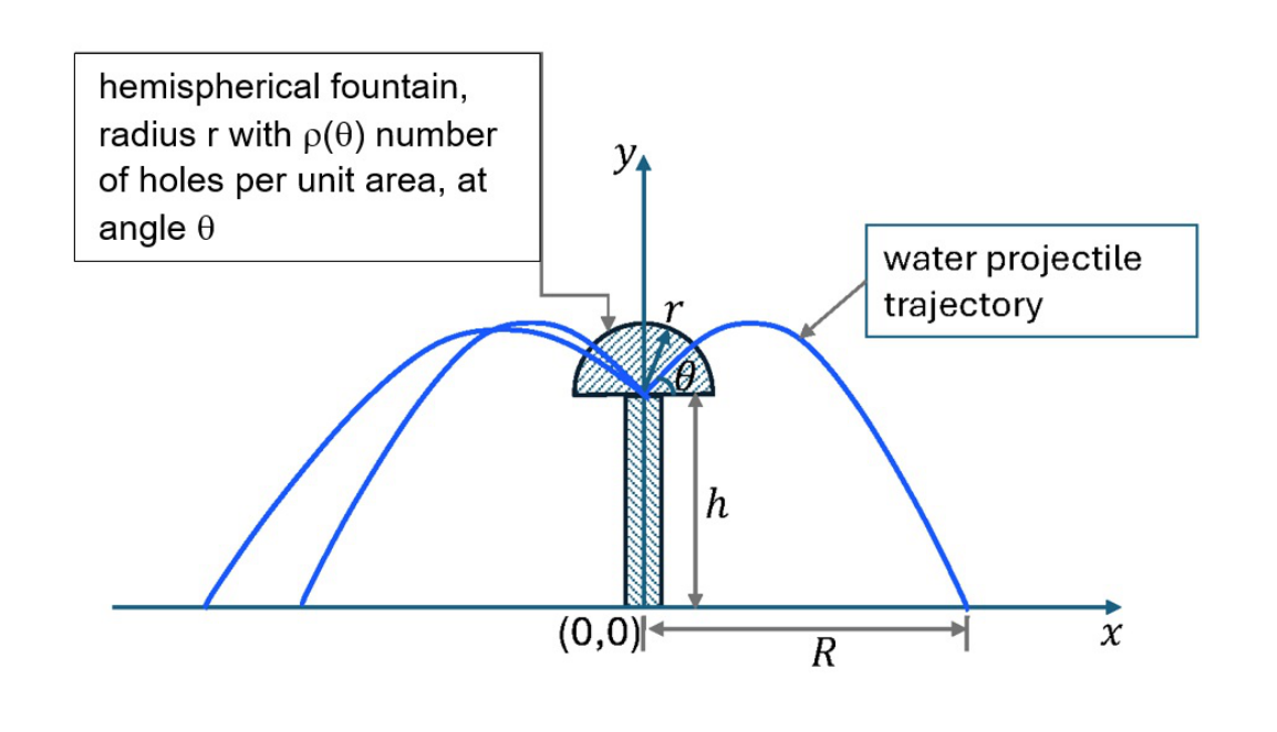Fig. 1: Schematic cross section of a hemispherical shaped fountain sprayer.

Part A: Uniformly Distributed Holes on the Surface of the Hemisphere (6.0 points)

First consider the holes distribution on the surface of the hemisphere to be uniform (i.e. $\rho (\theta )$ is a constant).

A.1 Express the instantaneous position $x(t)$ and $y(t)$ of a water element (can be treated as a stream of particles) launched at velocity $v_o$ at angle $\theta$. (0.5pt)

A.2 Derive the water trajectory relation $y=y(x,\theta )$ and express in a same type of trigonometric function (e.g. in terms of sine, cosine or tangent ONLY). Note that $\theta >0$. (1.0pt)

A.3 The envelope is the minimal boundary which encloses all water trajectories (i.e. no water will be found beyond this boundary). Derive the equation for the envelope for this system. Express your answer as $y(x)$. Sketch the envelope over the trajectories. (3.0pt)

A.4 Calculate the range $R=R(\theta )$ as a function of angle $\theta$. (1.0pt)

A.5 Letting $h\to 0$ in the range obtained in A.4, show that $R=\frac{v_o^2}{g}\sin 2\theta$. (0.5pt)

Part B: Non-Uniformly Distributed Holes on the Surface of the Hemisphere (4.0 points)

Now, consider the area of holes per unit area $\rho (\theta )$ to be non-uniformly distributed and depended on the angle $\theta$.

B.1 Using the results from part A.4 above, calculate the elemental area $d{A}_R$ of an annulus (ring) of radius $R$ and width $dR$ of the water hitting the ground. Express your answer in $R$, $R^{\prime }$ and $d\theta$. [hint: consider $R^{\prime }=\frac{dR}{d\theta }$.] (1.0pt)

B.2 Determine the relation for $\rho (\theta )$ that gives a uniform spray coverage pattern on the ground by considering elemental area on the hemisphere in proportional to the elemental area of the water spray on the ground. Express your answer in terms of $R$ and its derivative. [hint: consider condition where $R^{\prime }(\theta )>0$]. (1.0pt)

B.3 Letting $h=0$, calculate explicitly the relation for $\rho (\theta )$ that gives a uniform spray coverage pattern for $\theta <45^{\circ }$. (2.0pt)

Fonte: Testo (PDF) — p.1

Topic: Newtonian Mechanics, Mathematics Metodi: Kinematic Equations, Calculus-Integration, Vector Decomposition, Physical Modeling Competenze: Physical Reasoning, Mathematical Modeling, Diagrammatic Reasoning Objects: Projectile

Geometria della fontana d’acqua (30 punti)

Introduzione

I spruzzatori d’acqua si trovano in vari luoghi come allevamenti agricoli, parchi verdi o aree urbane per scopi funzionali o per installazioni di arte estetica. Si consideri un spruzzatore di fontana a forma emisfera di raggio $r$ all’altezza $h$ dal terreno come mostrato in un diagramma trasversale nella figura . 1. Il raggio di radio dell’emisfero deve essere piccolo rispetto al range $R$, quindi può essere considerato come fonte di punti. Tuttavia, ci sono $\rho (\theta )$ numero di fori per unità di superficie all’angolo $\theta$. L’acqua si spunta in tutte le direzioni alla stessa velocità iniziale $v_o$.

Fig. 1: Sezione trasversale schematica di un spruzzatore a fontana a forma emisfera.

**Parte A: Buchi uniformemente distribuiti sulla superficie dell’emisfero (6,0 punti) **

In primo luogo, si consideri che la distribuzione dei buchi sulla superficie dell’emisfero sia uniforme (cioè: $\rho (\theta )$ è una costante).

A.1 Esprimere la posizione istantanea $x(t)$ e $y(t)$ di un elemento idrico (può essere trattato come un flusso di particelle) lanciato a velocità $v_o$ all’angolo $\theta$. (0.5pt)

A.2 Derivare la relazione trajectoriale dell’acqua $y=y(x,\theta )$ ed esprimere in un stesso tipo di funzione trigonometrica (es. in termini di seno, cosino o tangente SOLO). Nota che $\theta >0$. (1.0pt)

A.3 L’envelope è il limite minimo che circonda tutte le traiettorie idriche (cioè: Non si troverà acqua oltre questo confine). Derivare l’equazione per l’involucro per questo sistema. Esprimere la risposta come $y(x)$. Segna la busta sulle traiettorie. (3.0pt)

A.4 Calcolare l’intervallo $R=R(\theta )$ come funzione dell’angolo $\theta$. (1.0pt)

A.5 Se si lascia $h\to 0$ nella gamma ottenuta in A.4, è indicato che $R=\frac{v_o^2}{g}\sin 2\theta$. (0.5pt)

**Parte B: Buchi distribuiti non uniformemente sulla superficie dell’emisfero (4,0 punti) **

Ora, si consideri che l’area dei fori per unità di area $\rho (\theta )$ sia distribuita in modo non uniforme e dipenda dall’angolo $\theta$.

B.1 Usando i risultati della parte A.4 di cui sopra, calcolare l’area elementare $d{A}_R$ di un annulo (anello) di raggio $R$ e la larghezza $dR$ dell’acqua che colpisce il suolo. Esprimi la tua risposta in $R$, $R^{\prime }$ e $d\theta$. [suggerimento: considerazione $R^{\prime }=\frac{dR}{d\theta }$.] *(1.0pt) *

B.2 Determinare la relazione per $\rho (\theta )$ che dà un modello uniforme di copertura dello spray sul suolo considerando l’area elementare sull’emisfero proporzionale all’area elementare dello spray di acqua sul suolo. Esprimere la risposta in termini di $R$ e della sua derivata. [suggerimento: considera la condizione in cui $R^{\prime }(\theta )>0$]. (1.0pt)

B.3 Permettere $h=0$, calcolare esplicitamente la relazione per $\rho (\theta )$ che dà un modello uniforme di copertura a spruzzo per $\theta <45^{\circ }$. (2.0pt)

Fonte: Testo (PDF) — p.1

Topic: Newtonian Mechanics, Mathematics Metodi: Kinematic Equations, Calculus-Integration, Vector Decomposition, Physical Modeling Competenze: Physical Reasoning, Mathematical Modeling, Diagrammatic Reasoning Objects: Projectile

Snell’s Law (30 points)

Introduction

When light is incident upon a dielectric interface, it will be reflected and refracted, depending on the incident angle of the light and the refractive indices of the dielectric media as shown in Fig. 1. The refraction of light is governed by the Snell’s law,

n_1 \sin\phi_1 = n_2 \sin\phi_2 \tag{1}

where $n_1$ and $n_2$ are the refractive indices of the lower and upper parts of the boundary, ${\varphi }_1$ and ${\varphi }_2$ are the angles that the light ray makes with the normal of the boundary.

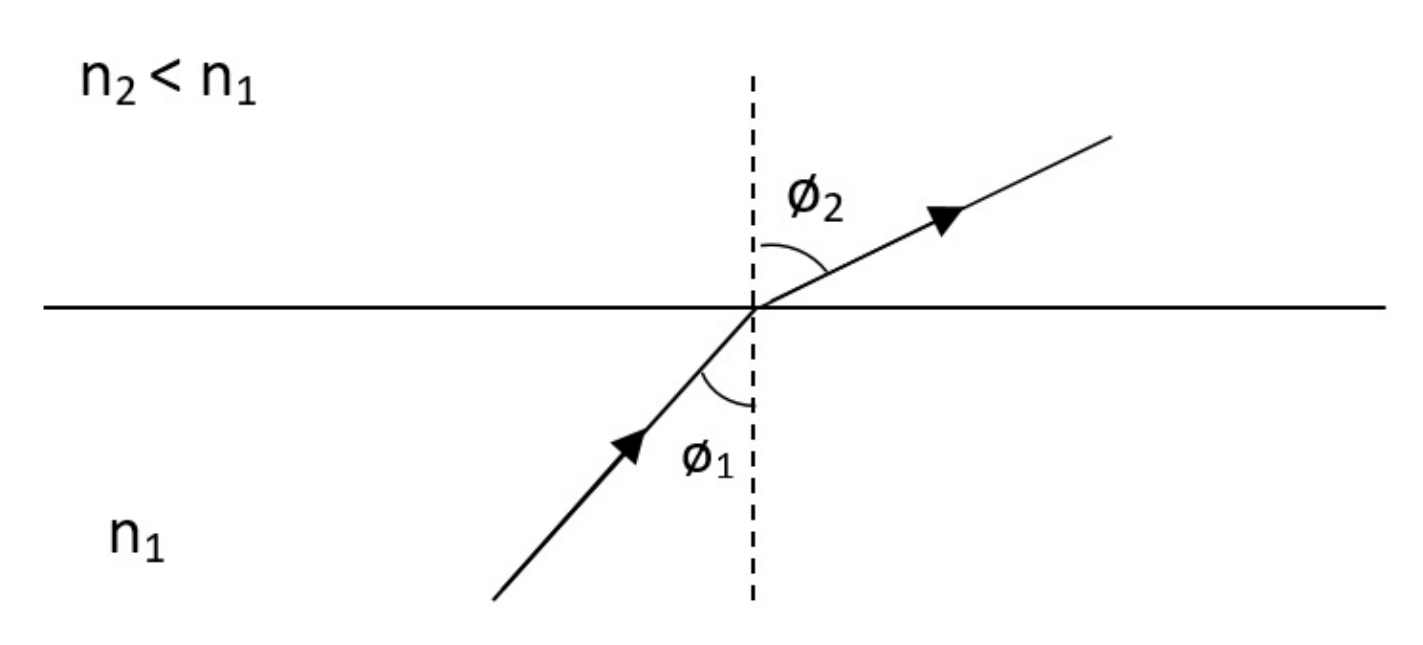Fig. 1: Refraction of light from a dielectric medium with refractive index $n_1$, to a second dielectric medium with refractive index $n_2$.

Part A: Light Propagation Through a Semi-Sphere (1.5 points)

Fig. 2 illustrates how light that consists of two rays with different colour, $a$ and $b$, is incident along the radius of a semi-sphere with refractive index $n_x$, in air, before being refracted at the bottom at an angle of ${\theta }_a$ and ${\theta }_b$, respectively.

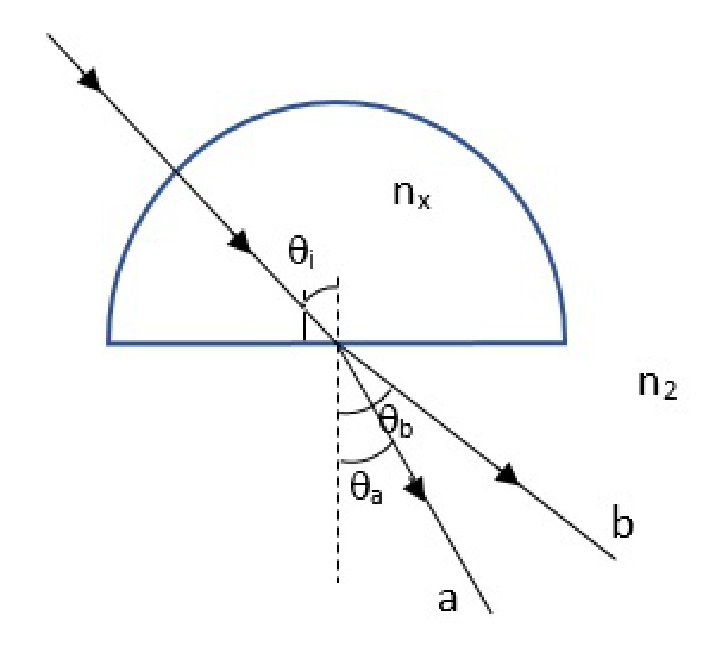Fig. 2: Light propagation through a semi-sphere.

A.1 Which ray ($a$ or $b$) propagates faster in the semi-sphere? Please provide justification. (0.5pt)

A.2 When the incident angle, ${\theta }_i$, is slowly increased to $45^{\circ }$, ray $b$ no longer exits the bottom of the semi-sphere. When ${\theta }_i$ is further increased to $50^{\circ }$, the same happens to ray $a$. What is the difference between the refractive index of ray $a$ and $b$ in the semi-sphere? (1.0pt)

Part B: Light Propagation Through a Cylindrical Rod (3.5 points)

A cylindrical rod has a refractive index of $n_1=1.50$. The rod is placed in air, with one end coated with a polymer with refractive index $n_2=1.40$, as shown in Fig. 3 below. Light is incident from the polymer into the rod at an angle, $\theta$. When $\theta$ is changed, there is an instance when light is totally reflected back to the polymer.

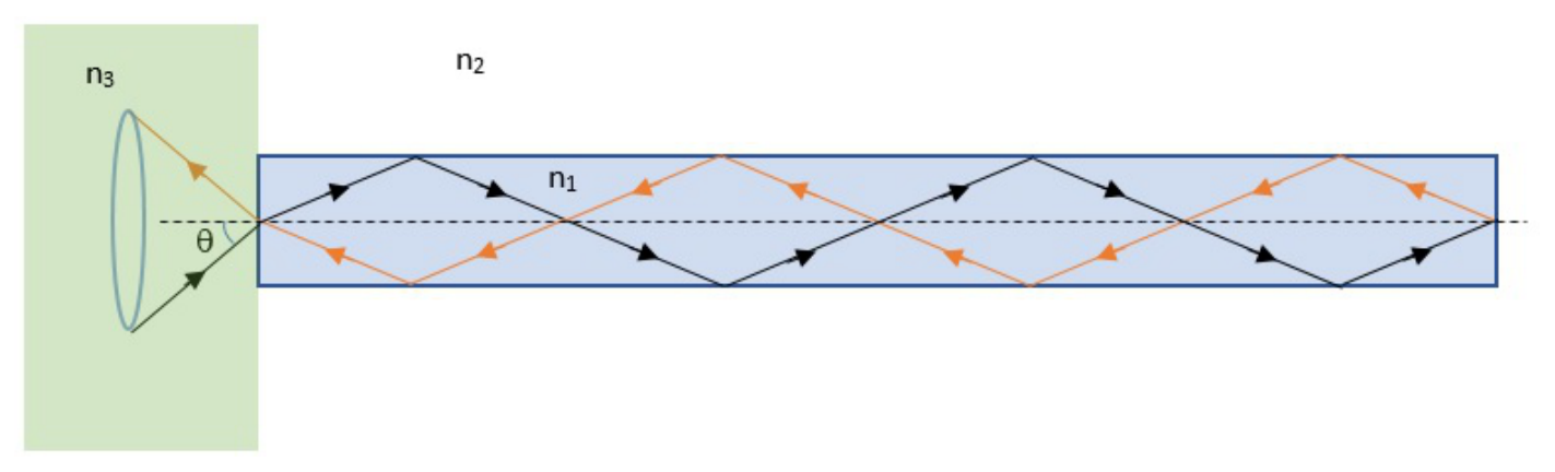Fig. 3: A cylindrical rod with one end coated with a polymer with refractive index $n_2$, where $n_2<n_1$.

B.1 Determine the range of incident angle, $\theta$, for this condition to happen. (2.0pt)

B.2 How does the condition in B.1 change,

    (i) if the other, open end of the rod is now coated with a thick layer of oil with refractive index of 1.60? (0.6pt)

    (ii) if the setup is placed in water with refractive index of 1.33? (0.9pt)

Part C: Light Propagation Through an Optical Fiber (5.0 points)

Optical fibre is formed by surrounding the medium with refractive index, $n_1$ with a lower refractive index medium, $n_2$, as shown in Fig. 4 below. The medium with refractive index, $n_1$ is known as the fibre cladding. The refractive index, $n_3$, is typically the refractive index of air ($n_3=1$).

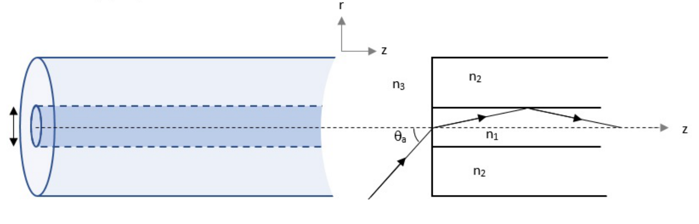Fig. 4: A schematic of an optical fibre and its cross section.

C.1 In order for light to propagate inside the optical fiber, it first needs to be coupled into the optical fiber. The maximum angle of the light incident at the end of the fiber, ${\theta }_a$, so that the light can be guided inside the fiber without being refracted out is related to the refractive indices of the fiber core and cladding. Consider a ray that propagates inside the optical fiber as shown in Fig. 4 below. Formulate the relationship between the angle, ${\theta }_a$ and the refractive indices. (2.0pt)

C.2 Optical fibers are not always aligned in a straight line but need to be bent to go through different spaces. Given the fiber core diameter of $50\mu \text{m}$, if the minimum bending radius on the optical fiber is $1.0\text{cm}$, how much will ${\theta }_a$ change? (2.6pt)

C.3 Given the refractive index of the fiber core and cladding is $1.45$ and $1.44$, respectively, what are the maximum angle of light incident for case C.1 and C.2 above, when the fiber is placed in air? (0.4pt)

Fonte: Testo (PDF) — p.1

Topic: Geometric Optics Metodi: Snell’s Law, Ray Tracing, Vector Decomposition Competenze: Physical Reasoning, Diagrammatic Reasoning, Mathematical Modeling Objects: Sphere, Rod

La legge di Snell

Introduzione

Quando la luce incide su un’interfaccia dielettrica, essa sarà riflessa e refrattata, a seconda dell’angolo di incidenza della luce e degli indici di rifrazione dei mezzi dielettrici come mostrato nella figura . 1. La rifrazione della luce è governata dalla legge di Snell,

n_1 \sin\phi_1 = n_2 \sin\phi_2 \tag{1}

se $n_1$ e $n_2$ sono gli indici di rifrazione delle parti inferiori e superiori del confine, ${\varphi }_1$ e ${\varphi }_2$ sono gli angoli che il raggio luminoso fa con la normalità del confine.

Fig. 1: Rifrazione della luce da un mezzo dielettrico con indice di rifrazione $n_1$ a un secondo mezzo dielettrico con indice di rifrazione $n_2$.

**Parte A: Propagazione della luce attraverso una semisfera (1.5 punti) **

Fig. 2 illustra come la luce costituita da due raggi di colore diverso, $a$ e $b$, si incontra nell’aria lungo il raggio di una semisfera con indice di rifrazione $n_x$, prima di essere rifracciata in fondo ad un angolo di ${\theta }_a$ e ${\theta }_b$, rispettivamente.

Fig. 2: Propagazione della luce attraverso una semisfera.

A.1 Quale raggio ($a$ o $b$) si propaga più velocemente nella semisfera? Per favore, fornisci una giustificazione. (0.5pt)

Quando l’angolo di incidenza, ${\theta }_i$, è lentamente aumentato a $45^{\circ }$, il raggio $b$ non esce più dal fondo della semisfera. Quando ${\theta }_i$ viene ulteriormente aumentato a $50^{\circ }$, lo stesso accade per il raggio $a$. Qual è la differenza tra l’indice di rifrazione del raggio $a$ e $b$ nella semisfera? (1.0pt)

**Parte B: Propagazione della luce attraverso una canna cilindrica (3,5 punti) **

Una canna cilindrica ha un indice di rifrazione $n_1=1.50$. La canna è collocata in aria, con un’estremità rivestita di un polimero con indice di rifrazione $n_2=1.40$, come mostrato nella figura . 3 di seguito. La luce si incide dal polimero nella canna ad un angolo $\theta$. Quando $\theta$ viene modificato, si verifica un caso in cui la luce si riflette completamente sul polimero.

Fig. 3: Una barra cilindrica con un’estremità rivestita di un polimero con indice di rifrazione $n_2$, dove $n_2<n_1$.

**B.1 ** Determina l’intervallo di angolo di incidenza, $\theta$, per ottenere questa condizione. (2.0pt)

B.2 Come cambia la condizione di B.1,

    **(i) ** se l’altra estremità aperta della canna è ora rivestita di uno spessore strato di olio con un indice di rifrazione di 1,60? (0.6pt)

    **(ii) ** se l’impianto è messo in acqua con un indice di rifrazione di 1,33? (0.9pt)

**Parte C: Propagazione della luce attraverso una fibra ottica (5,0 punti) **

La fibra ottica si forma circondando il mezzo con un indice di rifrazione $n_1$ con un indice di rifrazione inferiore $n_2$, come mostrato nella figura . 4 di seguito. Il mezzo con indice di rifrazione $n_1$ è noto come rivestimento a fibra. L’indice di rifrazione, $n_3$, è tipicamente l’indice di rifrazione dell’aria ($n_3=1$).

Fig. 4: Schema di una fibra ottica e della sua sezione trasversale.

**C.1 ** Per che la luce si diffonda all’interno della fibra ottica, è necessario prima accoppiarla nella fibra ottica. L’angolo massimo dell’incidente luminoso alla fine della fibra, ${\theta }_a$, in modo che la luce possa essere guidata all’interno della fibra senza essere refratta, è correlato agli indici di refraczione del nucleo della fibra e del rivestimento. Considerate un raggio che si propaga all’interno della fibra ottica come mostrato nella figura . 4 di seguito. Formulare la relazione tra l’angolo ${\theta }_a$ e gli indici di rifrazione. (2.0pt)

Le fibre ottiche non sono sempre allineate in linea retta, ma devono essere piegate per attraversare spazi diversi. Dato il diametro del nucleo della fibra $50\mu \text{m}$, se il raggio di piegatura minimo della fibra ottica è $1.0\text{cm}$, quanto cambierà ${\theta }_a$? (2.6pt)

C.3 Dato che l’indice di rifrazione del nucleo e del rivestimento di fibra è rispettivamente $1.45$ e $1.44$, qual è l’angolo massimo di incidente luminoso per i casi C.1 e C.2 di cui sopra, quando la fibra è messa in aria? (0.4pt)

Fonte: Testo (PDF) — p.1

Topic: Geometric Optics Metodi: Snell’s Law, Ray Tracing, Vector Decomposition Competenze: Physical Reasoning, Diagrammatic Reasoning, Mathematical Modeling Objects: Sphere, Rod

The First Discovered Quasar: Unveiling the Mysteries of the Astrophysical Source 3C 273 (30 points)

Part A: Moon’s Apparent Motion Against the Background Stars (1.8 points)

The Moon takes 27.3 days to complete 1 orbit of the Earth with respect to the stars, a period known as a sidereal month. Through a telescope, the moon’s motion is readily apparent, but to the eye, it requires careful observation over several hours to notice the Moon’s changing position. Remembering that 3600 arcseconds = 60 arcminutes = 1 degree then, through how many degrees, arcminutes, and arcseconds does the Moon move against the background of stars in

A.1 one hour? One minute? One second? (1.3pt)

A.2 How long does it take the Moon to move a distance equal to its own diameter on the sky? (Note: the angular diameter of the moon as viewed from Earth is 30 arcminutes) (0.5pt)

Part B: Using Lunar Occultations to Precisely Determine Radio Source Positions: The Case of 3C 273 (1.8 points)

In the late 1950s and early 1960s, radio position measurements with this precision were not available. While occultations had been used previously, Hazard was specifically interested in their ability to determine radio positions and structure with arcsecond precision. Such measurements were made in the optical reference frame thereby allowing reliable optical identifications. Hazard had noted that the strong Class II radio source 3C 273 would be hidden by the Moon (also known as occultation) several times during 1962 and 1963.

The 1962 August 5 occultation was undertaken at 410 and 136 MHz. Both disappearance and reappearance were observed and the disappearance record revealed the presence of two components, A and B, in the source. The disappearance on the right and the reappearance records on the left, at 410 MHz are plotted in Fig. 1.

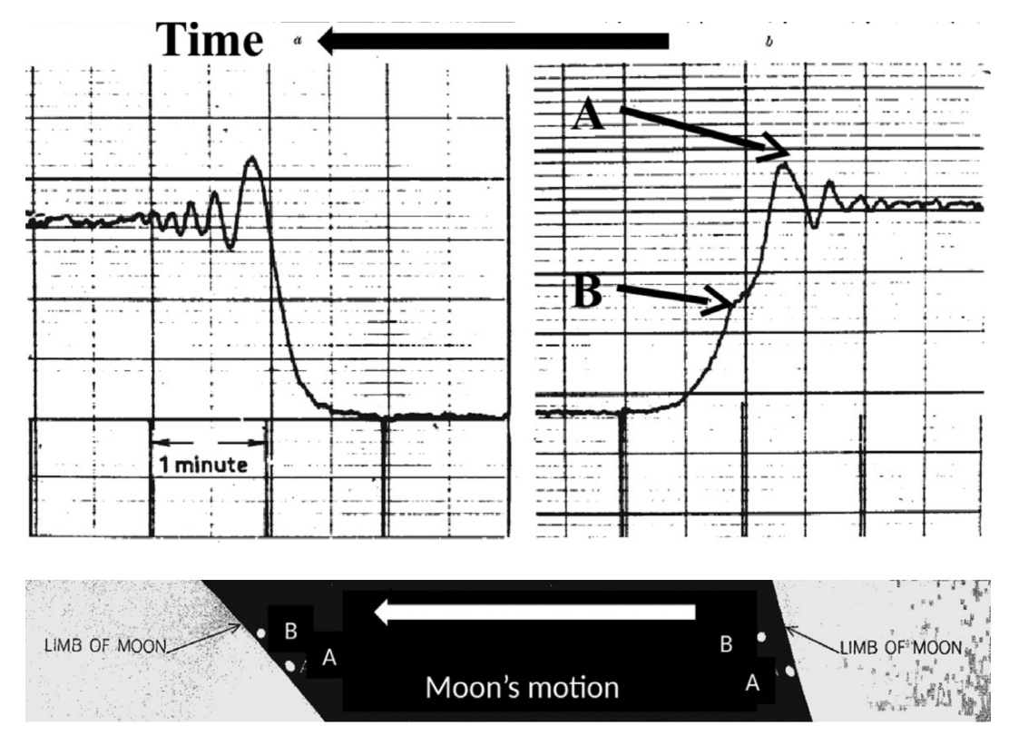Fig. 1: The 1962 August 5 disappearance and reappearance records at 410 MHz, taken from Hazard et al. (1963). Note that time increases from right to left, and that the Moon is also moving from right to left. The bottom panel shows the positions of source components A and B relative to the limb of the Moon at disappearance and reappearance.

B.1 What is causing the oscillation in the observed intensity? (0.6pt)

    A. The diffraction pattern of the telescope     B. Instabilities in the mount of the telescope     C. The features of the surface of the Moon     D. Earth’s atmospheric conditions

B.2 Why there is no extra bump for the B component in the left plot for the reappearance of the source? How does it help to understand the structure of the source? (0.6pt)

    A. The two components have been orbiting around the Moon.     B. Our line-of-sight has changed with respect to the two components.     C. Both components are aligned with the limb of the Moon when they reappear.     D. The time scales of the physics behind the luminosity of the two components were long enough to make one of them fade.

B.3 Based on your answer in A.1 to A.4, and the data in Fig. 1, estimate the approximate apparent (projected) angular separation between the two components of 3C 273. (0.6pt)

Part C: The Breakthrough Discovery of 3C 273’s True Nature (1.8 points)

In 1962, the year of these observations, Maarten Schmidt was working on the programme of optical identification and spectroscopy of the optical objects identified with radio sources. Whiteoak mentions as an afterthought that the ‘current Caltech thinking’ is that the potential 3C 273 identification is with a star and a strange jet. Given that no other bright star had been proposed as a radio source identification, he assumed that the bright magnitude 13 ‘star’ (magnitude accounts as a way to measure how bright a star is; the brighter the star, the smaller the number) was merely a confusing foreground very bright star. To obtain a spectrum of the faint jet, which he saw as by far the most likely identification, it was inevitable that the bright confusing star some arcseconds away would spill over into any spectrum of the jet he would obtain. To offset this, Maarten Schmidt had decided to first obtain a spectrum of this bright star. On the night of December 29, he managed to obtain a spectrum of the bright ‘star’ which showed some faint emission lines (Fig. 2), but with no obvious explanation in terms of any expected stellar lines. Only when Schmidt decided to compare the strange spectrum with the Balmer lines of hydrogen, things became clear:

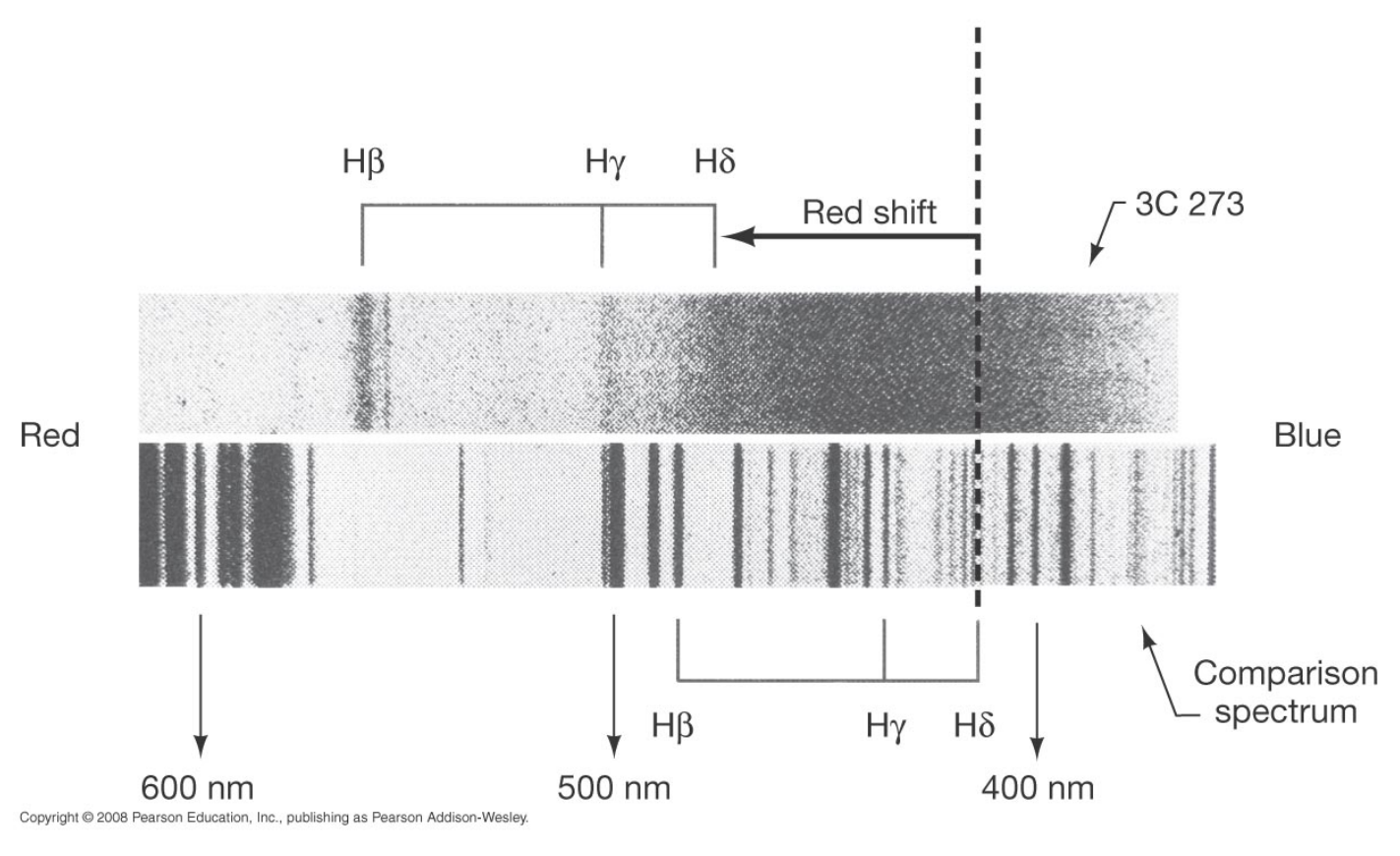Fig. 2: Optical spectrum of 3C 273 (top) together with a comparison laboratory spectrum (bottom).

C.1 Compare the wavelength ratios of the lines shown in Fig. 2. Based on these ratios, what is the redshift $z=\frac{\lambda -{\lambda }_0}{{\lambda }_0}$ of this source? (0.6pt)

C.2 Consider that this redshift is arising due to relativistic gravitational effects from the mass of the object. In this case, we can estimate the gravitational redshift as $z=\frac{1}{\sqrt{1-\frac{2GM}{c^{2}r}}}-1$. Prove that, whether you put 3C 273 at any distance (e.g, edge of the Milky Way, $r\sim 100\text{kpc}\sim 3\times 10^{21}\text{m}$; edge of the Solar System, $r\sim 100\text{AU}\sim 1.5\times 10^{13}\text{m}$), the mass of 3C 273 would be so large it would disrupt the entire galaxy / solar system. (0.6pt)

C.3 Hubble’s law states that the farther the galaxies, the faster they are moving away from Earth. The Hubble’s constant relates the recession velocity and the distance of those galaxies, and equal to $H\approx 75\text{km/s/Mpc}$. With this idea in mind, we can consider instead that the calculated redshift is due to the cosmological expansion, and we can approximate that $v\approx cz$. In that case, what is the distance of this object? Compare this with the size of the Milky Way. (0.6pt)

Part D: The Intrinsic Luminosity of the Radio Source 3C 273 (1.8 points)

The flux of the source 3C 273 has been measured across the radio spectrum and has been found to follow the equation $F_{\nu }\sim 25000{\nu }^{(-0.3)}$ Jy, where $\nu$ is the observed frequency in Hertz and a Jansky is defined as $1\text{Jy}=10^{-26}{\text{W m}}^{-2}{\text{Hz}}^{-1}$. Of course, since the source is radiating over a sphere of radius the distance from us, the intrinsic luminosity will be given by $L_{\nu }=4\pi d^2{F}_{\nu }$. With this,

D.1 What is the luminosity of the source per unit frequency? (help: $1\text{pc}=3.09\times 10^{16}\text{m}$) (0.6pt)

D.2 What is the total luminosity of the radio band (ie., from $10^7$ Hz to $10^{11}$ Hz)? (0.6pt)

D.3 How does the luminosity of 3C 273 compare with the luminosity of the Sun ($L_{sun}=3.82\times 10^{26}\text{W}$) and the Milky Way ($L_{MW}=1.5\times 10^{37}{L}_{sun}$) in the same frequency range? (0.6pt)

Part E: The Power Source of 3C 273 (1.4 points)

We have seen that the brightness of 3C 273 is too large for a single star, even for an entire galaxy. Therefore, there should be another mechanism, other than stars, producing all this power.

E.1 Check that the annihilation of matter with antimatter (e.g., $e^{+}+e^{-}\to 2\gamma$) would not explain this, since it would produce very energetic X-rays rays rather than optical and radio emission. (0.7pt)

E.2 Something that was immediately proposed was the accretion of matter into a supermassive black hole. Let’s check that potential energy can give all this energy: Consider that the black hole accretes one solar mass ($2\times 10^{30}$ kg) towards its Schwarzschild radius ($R_s=\frac{2GM}{c^2}$) every year. What is the power that can be obtained for the accretion? Would this be enough to explain the observations discussed in D1 to D3? (0.7pt)

Part F: Modern Observations and the Nature of 3C 273’s Components (1.4 points)

Modern images from various telescopes (see e.g., Fig. 3) have found that the two components A and B that were measured with the lunar occultation actually refer to a compact core, which hosts the black hole, and a jet that extends the distance that you calculated before. This jet is thought to be produced via acceleration of the accreted particles via the strong black hole magnetic field, in a similar way particles from the Solar wind hit the magnetic field of Earth to produce the auroras near the poles, but at much larger scale.

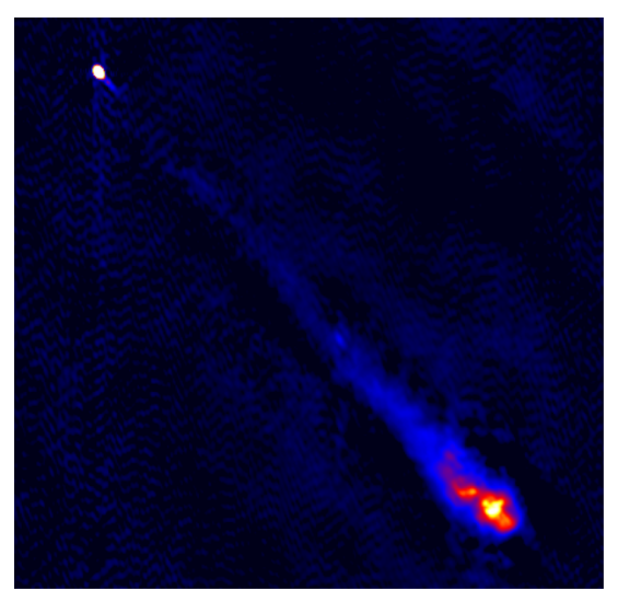Fig. 3: Radio image of 3C 273 taken with the MERLIN telescope.

The energy density required for the production of such jet can be written in terms of the magnetic fields as the sum of the particle energy density $U_e\sim B^{(-3/2)}$ and the magnetic energy density $U_B\sim B^2$.

F.1 Show that the minimum energy density is given by $\frac{U_e}{U_B}=\frac{4}{3}$. (0.7pt)

F.2 If we assume that the total power of the 3C 273 jet is given by half of the energy released by 3C 273 in one second calculated in D.1 and D.2, and the jet has a volume of $10^{45}{\text{m}}^3$, estimate the magnetic field of the jet. (hint: use that the magnetic permeability is $4\pi \times 10^{-7}{\text{T m A}}^{-1}$) (0.7pt)

Fonte: Testo (PDF) — p.1

Topic: Astrophysics, Special Relativity, Modern-Quantum Physics Metodi: Order-of-Magnitude Estimation, Mass-Energy Equivalence, Newton’s Law of Gravitation, Photon Energy Relation Competenze: Physical Reasoning, Estimation & Approximation, Unit Conversion Objects: Satellite, Star, Black Hole, Photon, Electron

Il primo quasar scoperto: rivelazione dei misteri della fonte astrofisica 3C 273

**Parte A: Movimento apparente della Luna contro le stelle di fondo (1.8 punti) **

La Luna richiede 27,3 giorni per completare 1 orbita della Terra rispetto alle stelle, un periodo noto come mese sidereale. Attraverso un telescopio, il movimento della luna è facilmente evidente, ma per l’occhio, richiede una attenta osservazione per diverse ore per notare la posizione cambiante della Luna. Ricordando che 3600 secondi d’arco = 60 minuti d’arco = 1 grado, quindi, attraverso quanti gradi, minuti d’arco e secondi d’arco la Luna si muove contro lo sfondo delle stelle in

**A.1 ** un’ora? - Un minuto? - Un secondo? - No. (1.3pt)

Quanto tempo ci vuole per spostare la Luna a una distanza pari al suo diametro nel cielo? (Nota: il diametro angolare della luna vista dalla Terra è di 30 minuti d’arco) *(0,5pt) *

**Parte B: Uso delle ocultazioni lunari per determinare con precisione le posizioni della fonte radio: il caso di 3C 273 (1,8 punti) **

Alla fine degli anni ‘50 e all’inizio degli anni ‘60, non erano disponibili misure di posizione radio con questa precisione. Mentre le occultazioni erano state usate in precedenza, Hazard era specificamente interessato alla loro capacità di determinare posizioni radio e struttura con precisione di arco secondo. Tali misurazioni sono state effettuate nel quadro di riferimento ottico, consentendo così un’identificazione ottica affidabile. Hazard aveva notato che la forte fonte radio di classe II 3C 273 sarebbe stata nascosta dalla Luna (noto anche come occultazione) diverse volte durante il 1962 e il 1963.

L’occultamento del 5 agosto 1962 è stato effettuato a 410 e 136 MHz. Sono state osservate sia la scomparsa che la riaparizione e il registro delle scomparse ha rivelato la presenza di due componenti, A e B, nella fonte. La scomparsa a destra e i registri di ripresa a sinistra, a 410 MHz, sono tracciati in Fig. 1.

Fig. 1: I registri di scomparsa e riapparimenti del 5 agosto 1962 a 410 MHz, prelevati da Hazard et al. (1963). Si noti che il tempo aumenta da destra a sinistra e che la Luna si muove anche da destra a sinistra. Il pannello inferiore mostra le posizioni dei componenti sorgenti A e B rispetto all’arto della Luna alla scomparsa e alla riapparenza.

**B.1 ** Cosa causa l’oscillazione nell’intensità osservata? (0.6pt)

   A. Il modello di diffrazione del telescopio     B. Instabilità nel monte del telescopio     C. Le caratteristiche della superficie lunare    D. Condizioni atmosferiche della Terra

Perché non c’è un’ulteriore urticaria per la componente B nella trama sinistra per la ripresa della fonte? Come aiuta a capire la struttura della fonte? (0.6pt)

   A. Le due componenti sono orbitate attorno alla Luna.     B. La nostra visione è cambiata rispetto a queste due componenti.     C. Entrambi i componenti sono allineati con l’arto della Luna quando riappare.    D. Le scale temporali della fisica dietro la luminosità dei due componenti erano abbastanza lunghe da far svanire uno di loro.

Basato sulla risposta di A.1 a A.4 e sui dati riportati nella figura . 1, stima la separazione angolare apparente (progettata) approssimativa tra i due componenti di 3C 273. (0.6pt)

**Parte C: La scoperta rivoluzionaria della vera natura di 3C 273 (1,8 punti) **

Nel 1962, anno delle osservazioni, Maarten Schmidt lavorava al programma di identificazione ottica e spettroscopia degli oggetti ottici identificati con fonti radio. Whiteoak menziona come un pensiero posteriore che il “attuale pensiero di Caltech” è che la potenziale identificazione 3C 273 è con una stella e un strano getto. Dato che nessuna altra stella brillante era stata proposta come fonte di identificazione radio, ha supposto che la stella brillante di magnitudo 13 (la magnitudo conta come un modo per misurare quanto brillante è una stella; più brillante è la stella, minore è il numero) fosse semplicemente una stella di primo piano confusa molto brillante. Per ottenere uno spettro del debole jet, che vedeva come l’identificazione più probabile, era inevitabile che la stella brillante confusa a pochi secondi d’arco si riversasse in qualsiasi spettro del jet che avrebbe ottenuto. Per compensare questo, Maarten Schmidt aveva deciso di ottenere prima uno spettro di questa stella brillante. Nella notte del 29 dicembre è riuscito a ottenere uno spettro della brillante “stella” che mostrava alcune sfavorevoli linee di emissioni (Fig. 2), ma senza spiegazioni ovvie in termini di linee stellari attese. Solo quando Schmidt decise di confrontare lo strano spettro con le linee di idrogeno di Balmer, le cose divennero chiare:

Fig. 2: Spettro ottico di 3C 273 (alto) insieme a uno spettro di confronto di laboratorio (infine).

C.1 Confronta i rapporti di lunghezza d’onda delle linee mostrate nella figura . 2. In base a questi rapporti, qual è il spostamento rosso $z=\frac{\lambda -{\lambda }_0}{{\lambda }_0}$ di questa fonte? (0.6pt)

**C.2 ** Si consideri che questo spostamento rosso sia dovuto agli effetti gravitazionali relativistici della massa dell’oggetto. In questo caso, possiamo stimare il spostamento di rossa gravitazionale come $z=\frac{1}{\sqrt{1-\frac{2GM}{c^{2}r}}}-1$. Prova che, se mettiamo 3C 273 a qualsiasi distanza (ad esempio, bordo della Via Lattea, $r\sim 100\text{kpc}\sim 3\times 10^{21}\text{m}$; bordo del Sistema Solare, $r\sim 100\text{AU}\sim 1.5\times 10^{13}\text{m}$), la massa di 3C 273 sarebbe così grande che interromperebbe l’intero sistema solare. (0.6pt)

La legge di Hubble afferma che più le galassie si allontanano dalla Terra, più velocemente si allontanano. La costante di Hubble relaziona la velocità di recessione e la distanza di queste galassie, ed è uguale a $H\approx 75\text{km/s/Mpc}$. Con questa idea in mente, possiamo considerare invece che il spostamento calcolato al rosso è dovuto all’espansione cosmologica, e possiamo approssimare che $v\approx cz$. In tal caso, qual è la distanza di questo oggetto? Confronta questo con le dimensioni della Via Lattea. (0.6pt)

**Parte D: L’illuminazione intrinseca della fonte radio 3C 273 (1,8 punti) **

Il flusso della fonte 3C 273 è stato misurato attraverso lo spettro radio e si è scoperto che segue l’equazione $F_{\nu }\sim 25000{\nu }^{(-0.3)}$ Jy, dove $\nu$ è la frequenza osservata in Hertz e un Jansky è definito come $1\text{Jy}=10^{-26}{\text{W m}}^{-2}{\text{Hz}}^{-1}$. Naturalmente, poiché la fonte irradia su una sfera di raggio la distanza da noi, la luminosità intrinseca sarà data da $L_{\nu }=4\pi d^2{F}_{\nu }$. Con questo,

D.1 Qual è la luminosità della sorgente per unità di frequenza? (aiuto: $1\text{pc}=3.09\times 10^{16}\text{m}$) *(0,6pt) *

D.2 Qual è la luminosità totale della banda radio (ad esempio, da $10^7$ Hz a $10^{11}$ Hz)? (0.6pt)

Come si confronta la luminosità di 3C 273 con la luminosità del Sole ($L_{sun}=3.82\times 10^{26}\text{W}$) e della Via Lattea ($L_{MW}=1.5\times 10^{37}{L}_{sun}$) nella stessa gamma di frequenze? (0.6pt)

**Parte E: La fonte di alimentazione di 3C 273 (1,4 punti) **

Abbiamo visto che la luminosità di 3C 273 è troppo grande per una singola stella, anche per un’intera galassia. Pertanto, dovrebbe esserci un altro meccanismo, diverso dalle stelle, che produca tutta questa potenza.

**E.1 ** Controllare che l’annientamento della materia con l’antimateria (ad esempio, $e^{+}+e^{-}\to 2\gamma$) non spieghino questo, poiché produrrebbe raggi X molto energetici piuttosto che emissioni ottiche e radio. (0.7pt)

Qualcosa che è stato immediatamente proposto è stato l’accrescimento di materia in un buco nero supermassiccio. Controlliamo se l’energia potenziale può dare tutta questa energia: Consideriamo che il buco nero accumula una massa solare ($2\times 10^{30}$ kg) verso il suo raggio Schwarzschild ($R_s=\frac{2GM}{c^2}$) ogni anno. Qual è la potenza che si può ottenere per l’accrescimento? Questo sarebbe sufficiente a spiegare le osservazioni discusse nelle lettere da D1 a D3? (0.7pt)

**Parte F: Osservazioni moderne e natura dei componenti di 3C 273 (1,4 punti) **

Immagini moderne da vari telescopi (vedi ad esempio Fig. 3) hanno scoperto che le due componenti A e B misurate con l’occultamento lunare si riferiscono in realtà a un nucleo compatto, che ospita il buco nero, e a un getto che estende la distanza che hai calcolato prima. Si pensa che questo getto sia prodotto attraverso l’accelerazione delle particelle accretate attraverso il forte campo magnetico del buco nero, in modo simile le particelle del vento solare colpiscono il campo magnetico della Terra per produrre le aurore vicino ai poli, ma su scala molto più grande.

Fig. 3: Immagine radio di 3C 273 presa con il telescopio MERLIN.

La densità energetica richiesta per la produzione di tale getto può essere scritta in termini di campi magnetici come la somma della densità energetica delle particelle $U_e\sim B^{(-3/2)}$ e della densità energetica magnetica $U_B\sim B^2$.

F.1 Indicare che la densità energetica minima è data da $\frac{U_e}{U_B}=\frac{4}{3}$. (0.7pt)

Se supponiamo che la potenza totale del getto 3C 273 sia data dalla metà dell’energia rilasciata da 3C 273 in un secondo calcolato in D.1 e D.2, e il getto abbia un volume di $10^{45}{\text{m}}^3$, stimare il campo magnetico del getto. (suggetta: utilizzare che la permeabilità magnetica sia $4\pi \times 10^{-7}{\text{T m A}}^{-1}$) *(0,7pt) *

Fonte: Testo (PDF) — p.1

Topic: Astrophysics, Special Relativity, Modern-Quantum Physics Metodi: Order-of-Magnitude Estimation, Mass-Energy Equivalence, Newton’s Law of Gravitation, Photon Energy Relation Competenze: Physical Reasoning, Estimation & Approximation, Unit Conversion Objects: Satellite, Star, Black Hole, Photon, Electron