APhO 2025 — Teorica

Precession of the Earth’s axis (10.0 points)

Introduction

It has been known since ancient times that the Earth’s axis of rotation precesses. That is, the axis itself rotates around the line perpendicular to the ecliptic plane, i.e., the plane containing the Earth’s orbit around the Sun. Ancient Greek astronomer Hipparchus concluded that the annual angular displacement of the axis was approximately $45^{\prime \prime }$ (seconds of arc), which would imply that the period of axial precession is around $29000$ years. Modern measurements indicate that the period is approximately $25800$ years. In this problem, you are asked to investigate this phenomenon using Newtonian mechanics.

You may need the following constants:

• gravitational constant: $G=6.67\times 10^{-11}\text{N}{\text{m}}^2/{\text{kg}}^2$
• average radius of Earth: $R=6.371\times 10^6\text{m}$
• mass of the Earth: $M_E=5.972\times 10^{24}\text{kg}$
• average distance of the Sun from the Earth: $d_{SE}=1.496\times 10^{11}\text{m}$
• mass of the Sun: $M_S=1.989\times 10^{30}\text{kg}$
• average distance of the Moon from the Earth: $d_{ME}=3.844\times 10^8\text{m}$
• mass of the Moon: $M_M=7.348\times 10^{22}\text{kg}$
• Earth’s axial tilt: $\alpha =23.5^{\circ }$

Part A. The shape of the Earth (1.0 points)

The Sun and the Moon exert nonzero torques on the Earth because of its non-spherical shape, giving rise to its axial precession. The main reason behind the Earth’s non-spherical shape is the centrifugal force caused by the Earth’s rotation about its axis. The tectonic plates located on the Earth’s surface have deformed over millions of years to minimize stress within them. Therefore, as an approximation, let us model the Earth as a large liquid droplet of uniform density whose shape is determined by centrifugal and gravitational forces. In this model, the Earth’s surface is an oblate spheroid (ellipsoid of revolution) characterized by the polar radius $R_p$ and the equatorial radius $R_e$ (see Figure A.1).

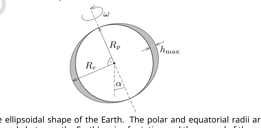
Figure A.1. The ellipsoidal shape of the Earth. The polar and equatorial radii are indicated. $\alpha =23.5^{\circ }$ is the angle between the Earth’s axis of rotation and the normal of the ecliptic plane.

The difference between the equatorial and polar radii of the Earth, $h_{\max }=R_e-R_p$ is much smaller than the average radius $R=(R_e+R_p)/2$. Up to a dimensionless factor, the value of $h_{\max }$ can be expressed in terms of the angular speed of the Earth’s rotation $\omega$, its mass $M_E$ and average radius $R$ as

$h_{\max }\propto G^{-1}{\omega }^{\beta }{M}_E^{\gamma }{R}^{\delta },$

where $G$ is the gravitational constant, and $\beta$, $\gamma$ and $\delta$ are constant exponents.

A.1 (0.8 pt) Find the values of exponents $\beta$, $\gamma$ and $\delta$.

A.2 (0.2 pt) Calculate the numerical value of $h_{\max }$ assuming that the dimensionless factor in the relation given above equals $1$.

Regardless of whether you were able to find $h_{\max }$ in part A.2., use the empirical value $h_{\max }=21\text{km}$ in the following questions.

Part B. The time-averaged gravitational field of the Sun (3.2 points)

To see why the Sun exerts a nonzero torque (with respect to the center of the Earth) on our planet, consider Figure B.1 below. The difference in distance from the Sun causes the gravitational force $F_1$ to be greater than its counterpart $F_2$.

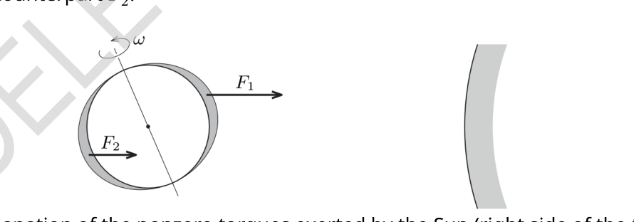
Figure B.1. Explanation of the nonzero torques exerted by the Sun (right side of the figure) on the Earth (left side).

The magnitude of this torque acting on the Earth varies continuously during the year. In the position shown in Figure B.1, the torque is maximal, a quarter of a year later, due to symmetry, the torque becomes zero. After half a year, it reaches the maximum again, three-quarters of a year later it is zero once again, and so on. Since the period of axial precession is much larger than one year, this time-dependent torque can be approximated well by its one-year average.

To calculate the average torque exerted by the Sun on the Earth, let us determine first the time average of the gravitational field generated by the Sun in the vicinity of the Earth. This average can be calculated as the field of a uniformly dense mass ring, a Sun ring, whose mass equals the mass of the Sun $M_S$ and whose radius equals the average distance between the Sun and the Earth $d_{SE}$ (see Figure B.2).

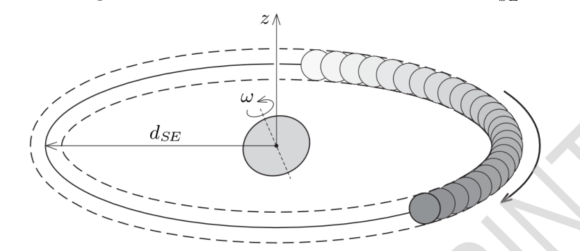
Figure B.2. Time averaging is equivalent to uniformly spreading the Sun along the circle of radius $d_{SE}$.

Let our cylindrical coordinate system have the origin at the center of the Earth, and let the $z$ axis be perpendicular to the ecliptic plane (i.e. the plane of the ring). The axis of rotation of the Earth makes an angle of $\alpha =23.5^{\circ }$ with the $z$ axis.

B.1 (1.0 pt) Find the direction and magnitude of the gravitational field generated by the Sun ring at a point on the $z$ axis. Write your answer in terms of $M_S$, $d_{SE}$, and the coordinate $z$. Assume that $|z|\ll d_{SE}$.

B.2 (2.2 pt) Find the direction and magnitude of the gravitational field generated by the Sun ring at a point in the ecliptic plane whose distance from the origin is $r$. Assume that $r\ll d_{SE}$.

Part C. The torque acting on the Earth (2.6 points)

In this section, you are asked to determine the torque exerted on the Earth due to the gravitational field obtained in Part B. For simplicity, consider the Earth as a rigid body with homogeneous mass distribution. Let us take into account that the rotational ellipsoid can be imagined as if we removed excess parts from a sphere with the equatorial radius of Earth $R_e$ (see Figure C.1).

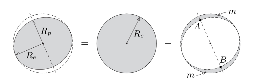
Figure C.1. The ellipsoidal shape of the Earth can be imagined as if the excess parts were removed from a complete sphere of radius $R_e$.

C.1 (0.8 pt) Find the mass $m$ of one of the two excess regions indicated in Figure C.1. Express your answer in terms of $h_{\max }$, the mass of the Earth $M_E$, and its polar radius $R_p$.

It can be shown that the torque acting on the excess regions is equivalent to the torque acting on two point masses, each with a mass equal to $2m/5$, positioned at the endpoints $A$ and $B$ of the polar diameter (see Figure C.1).

C.2 (1.8 pt) Given this idea, find the torque $\tau$ exerted by the Sun ring on the Earth. Express your answer in terms of $M_E$, $M_S$, $d_{SE}$, $R$ (the average radius), $h_{\max }$ and the angle $\alpha$. You can use that $h_{\max }\ll R$.

Part D. Angular speed of the precession of the Earth’s axis (2.0 points)

The Earth’s axis of rotation moves very slowly around the $z$ axis in a conical motion. That is, it precesses.

D.1 (1.8 pt) Give an expression for the period $T_1$ of precession of the Earth’s axis. Express your answer in terms of $M_S$, $d_{SE}$, the angular speed $\omega$ of the Earth’s rotation, $h_{\max }$, $R$ and $\alpha$.

D.2 (0.2 pt) Calculate the precession period $T_1$ in years.

Part E. The effect of the Moon (1.2 points)

The value obtained in Part D is much larger than the observed value. The reason for this is that so far we have only considered the torque exerted by the Sun, and neglected the effect of the Moon. In the following calculations, assume that the Moon’s orbit is in the ecliptic plane, and that the orbit of the Moon around the Earth is a circle of radius $d_{ME}$. Let us denote the mass of the Moon by $M_M$ and the period of precession in this modified model by $T_2$.

E.1 (1.0 pt) By what factor $T_2/T_1$ does the period of precession of the Earth’s axis change if we also take into account the torque exerted by the Moon? Give your answer in terms of $d_{ME}$, $d_{SE}$, $M_S$ and $M_M$.

E.2 (0.2 pt) By substituting the data, calculate the period of precession $T_2$ in years.

Fonte: Testo (PDF) — p.1 Topic: Gravitation, Rotational Dynamics Metodi: Newton’s Law of Gravitation, Torque & Angular Momentum Analysis, Dimensional Analysis, Symmetry Argument Competenze: Physical Reasoning, Mathematical Modeling Objects: Planet, Star, Satellite, Droplet

---

Precessione dell’asse della Terra (10,0 punti)

Introduzione

È noto fin dall’antichità che l’asse della rotazione della Terra procede. Cioè, l’asse stesso ruota intorno alla linea perpendicolare al piano eclittico, cioè il piano che contiene l’orbita terrestre intorno al Sole. L’antico astronomo greco Hipparco concluse che il spostamento angolare annuale dell’asse era approssimativamente $45^{\prime \prime }$ (secondi di arco), il che implicerebbe che il periodo di precisione assiale è intorno $29000$ anni. Le misurazioni moderne indicano che il periodo è di circa $25800$ anni. In questo problema, vi viene chiesto di indagare su questo fenomeno utilizzando la meccanica newtoniana.

Potresti aver bisogno delle seguenti costanti:

• costante gravitazionale: $G=6.67\times 10^{-11}\text{N}{\text{m}}^2/{\text{kg}}^2$
• raggio medio della Terra: $R=6.371\times 10^6\text{m}$
• massa della Terra: $M_E=5.972\times 10^{24}\text{kg}$
• distanza media del Sole dalla Terra: $d_{SE}=1.496\times 10^{11}\text{m}$
• massa del Sole: $M_S=1.989\times 10^{30}\text{kg}$
• distanza media della Luna dalla Terra: $d_{ME}=3.844\times 10^8\text{m}$
• massa della Luna: $M_M=7.348\times 10^{22}\text{kg}$
• Inclinazione assiale della Terra: $\alpha =23.5^{\circ }$

Parte A. Forma della Terra (1,0 punti)

Il Sole e la Luna esercitano torque non zero sulla Terra a causa della sua forma non sferica, dando origine alla sua precessione asiale. La ragione principale della forma non sferica della Terra è la forza centrifugata causata dalla rotazione della Terra intorno al suo asse. Le placche tettoniche situate sulla superficie terrestre si sono deformate nel corso di milioni di anni per ridurre al minimo lo stress all’interno. Quindi, come approssimazione, modelliamo la Terra come una grande goccia liquida di densità uniforme la cui forma è determinata dalle forze centrifuga e gravitazionale. In questo modello, la superficie terrestre è uno sferoide oblato (ellipsoide di rivoluzione) caratterizzato dal raggio polare $R_p$ e dal raggio equatoriale $R_e$ (vedi Figura A.1).

Figura A.1. La forma ellipssoidale della Terra. I raggi polari e equatoriali sono indicati. $\alpha =23.5^{\circ }$ è l’angolo tra l’asse di rotazione della Terra e la normalità del piano eclittico.

La differenza tra i raggi equatoriali e polari della Terra, $h_{\max }=R_e-R_p$, è molto inferiore al raggio medio $R=(R_e+R_p)/2$. Fino a un fattore senza dimensioni, il valore di $h_{\max }$ può essere espresso in termini di velocità angolare della rotazione terrestre $\omega$, massa $M_E$ e raggio medio $R$ come

$h_{\max }\propto G^{-1}{\omega }^{\beta }{M}_E^{\gamma }{R}^{\delta },$

dove $G$ è la costante gravitazionale e $\beta$, $\gamma$ e $\delta$ sono esponenti costanti.

**A.1 ** *(0,8 pt) * Trova i valori degli esponenti $\beta$, $\gamma$ e $\delta$.

A.2 (0,2 pt) Calcolare il valore numerico di $h_{\max }$ supponendo che il fattore dimensionato nella relazione indicata sopra sia uguale a $1$.

Indipendentemente dal fatto che si sia riuscito a trovare $h_{\max }$ nella parte A.2., utilizzare il valore empirico $h_{\max }=21\text{km}$ nelle seguenti domande.

Parte B. Il campo gravitazionale medio temporale del Sole (3,2 punti)

Per capire perché il Sole esercita una coppia non zero (rispetto al centro della Terra) sul nostro pianeta, considera la Figura B.1 qui sotto. La differenza di distanza dal Sole fa sì che la forza gravitazionale $F_1$ sia maggiore della sua controparte $F_2$.

Figura B.1. Spiegazione dei coppi non zero esercitati dal Sole (destra parte della figura) sulla Terra (sinistra).

La magnitudo di questa coppia che agisce sulla Terra varia continuamente durante l’anno. Nella posizione mostrata nella figura B.1, la coppia è massima, un quarto di anno dopo, a causa della simmetria, la coppia diventa zero. Dopo mezzo anno, raggiunge nuovamente il massimo, tre quarti di un anno dopo, torna a zero, e così via. Poiché il periodo di precisione assiale è molto più grande di un anno, questo coppia a seconda del tempo può essere approssimato bene dalla sua media di un anno.

Per calcolare la coppia media esercitata dal Sole sulla Terra, determineremo prima la media temporale del campo gravitazionale generato dal Sole nelle vicinanze della Terra. Questa media può essere calcolata come il campo di un anello di massa uniformemente denso, un anello solare, la cui massa è uguale alla massa del Sole $M_S$ e il cui raggio è uguale alla distanza media tra il Sole e la Terra $d_{SE}$ (vedere figura B.2).

Figura B.2. La media del tempo equivale a una distribuzione uniforme del Sole lungo il cerchio di raggio $d_{SE}$.

Che il nostro sistema di coordinate cilindriche abbia l’origine al centro della Terra, e che l’asse $z$ sia perpendicolare al piano eclittico (cioè il piano dell’anello). L’asse di rotazione della Terra fa un angolo di $\alpha =23.5^{\circ }$ con l’asse $z$.

**B.1 ** *(1.0 pt) * Trova la direzione e la grandezza del campo gravitazionale generato dall’anello solare in un punto sull’asse $z$. Scrivi la tua risposta in termini di $M_S$, $d_{SE}$ e la coordinata $z$. Supponiamo che $|z|\ll d_{SE}$.

B.2 *(2.2 pt) * Trova la direzione e la grandezza del campo gravitazionale generato dall’anello solare in un punto del piano eclittico la cui distanza dall’origine è $r$. Supponiamo che $r\ll d_{SE}$.

Parte C. La coppia che agisce sulla Terra (2,6 punti)

In questa sezione, vi viene chiesto di determinare la coppia esercitata sulla Terra a causa del campo gravitazionale ottenuto nella parte B. Per semplicità, considera la Terra come un corpo rigido con distribuzione di massa omogenea. Prendiamo in considerazione che l’ellissoide rotazionale può essere immaginato come se rimuovessimo le parti in eccesso da una sfera con il raggio equatoriale della Terra $R_e$ (vedi Figura C.1).

Figura C.1. La forma ellipssoidale della Terra può essere immaginata come se le parti in eccesso fossero state rimosse da una sfera completa di raggio $R_e$.

C.1 (0,8 pt) Trova la massa $m$ di una delle due regioni in eccesso indicate nella figura C.1. Esprimete la vostra risposta in termini di $h_{\max }$, massa della Terra $M_E$ e raggio polare $R_p$.

È possibile dimostrare che la coppia che agisce sulle regioni in eccesso è equivalente alla coppia che agisce su due masse puntine, ciascuna con una massa pari a $2m/5$, posizionata ai punti terminali $A$ e $B$ del diametro polare (vedi figura C.1).

C.2 *(1.8 pt) * Dato questo punto di vista, trovi la coppia $\tau$ esercitata dall’anello solare sulla Terra. Esprimere la risposta in termini di $M_E$, $M_S$, $d_{SE}$, $R$ (radius medio), $h_{\max }$ e angolo $\alpha$. Puoi usare questo $h_{\max }\ll R$.

Parte D. Velocità angolare della precisione dell’asse terrestre (2.0 punti)

L’asse di rotazione della Terra si muove molto lentamente intorno all’asse $z$ in movimento conico. Cioè, si precede.

D.1 (1.8 pt) Indicare un’espressione per il periodo $T_1$ di precisione dell’asse terrestre. Esprimere la risposta in termini di $M_S$, $d_{SE}$, velocità angolare $\omega$ della rotazione terrestre, $h_{\max }$, $R$ e $\alpha$.

**D.2 ** *(0,2 pt) * Calcolare il periodo di precessione $T_1$ in anni.

Parte E. L’effetto della Luna (1.2 punti)

Il valore ottenuto nella parte D è molto più grande del valore osservato. La ragione è che finora abbiamo considerato solo la coppia esercitata dal Sole, e abbiamo trascurato l’effetto della Luna. Nei seguenti calcoli, supponiamo che l’orbita della Luna sia nel piano eclittico e che l’orbita della Luna attorno alla Terra sia un cerchio di raggio $d_{ME}$. Indichiamo la massa della Luna con $M_M$ e il periodo di precessione in questo modello modificato con $T_2$.

**E.1 ** *(1.0 pt) * Con quale fattore $T_2/T_1$ cambia il periodo di precesione dell’asse terrestre se si tiene conto anche della coppia esercitata dalla Luna? Rispondi in termini di $d_{ME}$, $d_{SE}$, $M_S$ e $M_M$.

E.2 *(0,2 pt) * Sostituendo i dati, calcolare il periodo di precisione $T_2$ in anni.

Fonte: Testo (PDF) — p.1 Topic: Gravitation, Rotational Dynamics Metodi: Newton’s Law of Gravitation, Torque & Angular Momentum Analysis, Dimensional Analysis, Symmetry Argument Competenze: Physical Reasoning, Mathematical Modeling Objects: Planet, Star, Satellite, Droplet

---

Waves and Phase Transitions in Spin Systems (10.0 points)

Introduction

In classical physics, angular momentum arises from the motion of an object around an axis — whether it be a spinning top, a rotating planet, or an orbiting electron in the atom. However, in quantum physics, fundamental particles possess an intrinsic and quantized form of angular momentum called spin. This property plays a crucial role in various physical phenomena, ranging from materials properties, such as magnetism, to modern applications, such as quantum computing.

In this problem we will treat spin classically, which will lead to some qualitatively correct results. You will explore the physics of spin systems through spin-spin interactions, evolution under magnetic fields, and statistical physics to understand the emergence of spin waves and phase transitions in magnets.

Useful information:

$\cosh (x)\equiv \frac{e^x+e^{-x}}{2},\sinh (x)\equiv \frac{e^x-e^{-x}}{2},\tanh (x)\equiv \frac{\sinh (x)}{\cosh (x)}\approx x-\frac{1}{3}{x}^3\text{ for }|x|\ll 1$

The magnetic field due to a magnetic dipole of moment $\vec{\mu }$ at a position $\vec{r}$ away from it is given by (${\mu }_0$ is the vacuum permeability):

\vec{B} = \frac{\mu_o}{4\pi}\left( \frac{3(\vec{\mu} \cdot \vec{r})\,\vec{r}}{r^5} - \frac{\vec{\mu}}{r^3} \right) \tag{1}

Part A. Precession and interactions of magnetic dipoles (1.2 points)

Consider a ring of radius $R$, total mass $M$, and charge $Q>0$ distributed uniformly. The ring rotates with an angular speed $\omega$ around a perpendicular axis that passes through its center of mass.

A.1 (0.3 pt) It is possible to write the ring’s magnetic moment $\vec{\mu }$ in terms of its angular momentum $\vec{L}$ as $\vec{\mu }=\gamma \vec{L}$. Find the constant $\gamma$, called the gyromagnetic ratio, of this system in terms of $Q$ and $M$.

The ring is placed in a weak uniform magnetic field $\vec{B}=B\hat{z}$, making an angle $\theta$ with $\vec{\omega }$, see Figure A.1.

Figure A.1.

A.2 (0.4 pt) Find the angular frequency ${\omega }_L$ of the angular momentum precession (the so-called Larmor frequency) due to the external magnetic field in terms of $B$ and $\gamma$. Take the positive direction to be counter-clockwise with respect to $+z$.

Now we turn off the external magnetic field and place an identical ring at a horizontal distance $d\gg R$ from the original ring such that the magnetic moment of the new ring ${\vec{\mu }}_2$ makes an angle $\theta$ with ${\vec{\mu }}_1$, see Figure A.2.

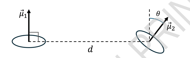
Figure A.2.

A.3 (0.5 pt) The magnetic interaction energy between the two rings can be written as $U=J_0{\vec{L}}_1\cdot {\vec{L}}_2$, where $J_0$ is a constant and ${\vec{L}}_i$ is the angular momentum of the $i$th ring. Find $J_0$ in terms of $\gamma$, $d$ and fundamental constants.

Part B. Spin Waves (4.5 points)

In what follows we investigate the dynamics of spins. A spin is a particle with intrinsic angular momentum $\vec{S}$, which has an associated magnetic moment $\vec{\mu }$ related to $\vec{S}$ via the gyromagnetic ratio as in Part A.1, $\vec{\mu }=\gamma \vec{S}$.

The magnetic dipoles of two spins interact with each other. However, this interaction is negligible compared to another interaction arising from a quantum mechanical origin, which is not present in classical systems. Interestingly, the energy associated with this quantum interaction has the same form which we found in Part A.3, scaling with ${\vec{S}}_1\cdot {\vec{S}}_2$, albeit with the opposite sign.

Now we will look at a very long chain of spins. The positions of the spins are fixed along the $x$-axis, with a distance $a$ separating them, see Figure B.1. We will approximate the total energy of the system by considering the interactions between nearest neighbors only, so that the energy can be written as

$E=-J{\sum }_i{\vec{S}}_i\cdot {\vec{S}}_{i+1}$

where $J>0$ is the interaction strength, and ${\vec{S}}_i$ is the spin angular momentum vector of the $i$th dipole, with magnitude $S$. The spin vectors are free to rotate in three dimensions. Notice that the sign of the energy is different from the last part. This interaction is purely quantum mechanical.

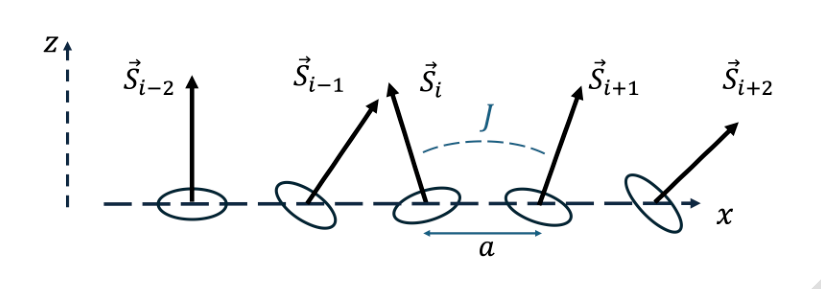
Figure B.1.

B.1 (0.3 pt) The energy terms containing ${\vec{S}}_i$ in the sum above can be viewed as the interaction energy between an effective magnetic field ${\vec{B}}_{i,\text{eff}}$ and the magnetic moment of ${\vec{S}}_i$. Find ${\vec{B}}_{i,\text{eff}}$ and express your answer in terms of $J$, the gyromagnetic ratio $\gamma$, and other spins ${\vec{S}}_j$ (specify the indices $j$ in relation to $i$).

B.2 (0.3 pt) Using the concept of effective magnetic field, express the rate of change of the $i$th spin vector, $d{\vec{S}}_i/dt$, in terms of $J$, ${\vec{S}}_i$, and other spins ${\vec{S}}_j$ (specify the indices $j$ in relation to $i$).

For the rest of Part B, assume that the system is highly magnetized along the $z$ direction, so we can use the approximations $S_{i,z}\approx S$ and $d{S}_{i,z}/dt\approx 0$ for each spin, see Figure B.2. In this regime, the set of equations describing the spins time evolution is satisfied by a traveling wave solution for $S_{i,x}$ and $S_{i,y}$ characterized by a wave vector $k$ and angular frequency $\omega$.

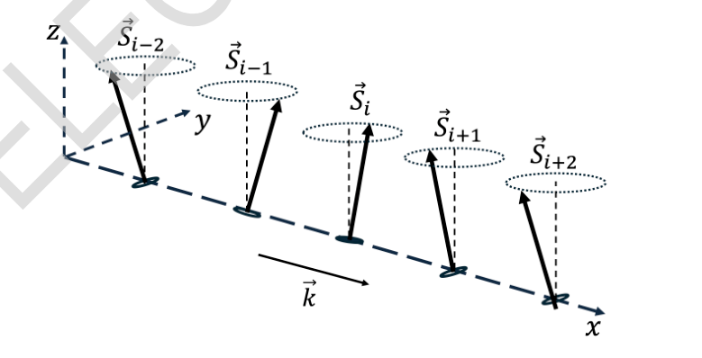
Figure B.2.

B.3 (2.0 pt) Find the relationship between $\omega$ and $k$ (known as the dispersion relation, $\omega (k)$) for the spin waves in terms of $J$, $S$ and $a$. Hint: express the position of the $i$th spin as $x=a\cdot i$.

The spin wave described above carries energy and momentum. At low energies, the relation between its energy and momentum resembles that of a massive classical particle with an effective mass $m_{\text{eff}}$, a concept known as a quasi-particle.

B.4 (0.6 pt) For small $k$ ($k\ll 1/a$), find the effective mass $m_{\text{eff}}$ of the spin wave. Express your answer in terms of $J$, $S$, $a$ and fundamental constants.

Spin waves can be experimentally probed using inelastic neutron scattering. Although neutrons have zero net charge, they have a finite spin, allowing them to interact with other spins.

B.5 (1.3 pt) Suppose that initially, all the spins in the chain are pointing along the $z$ direction. A neutron with low energy travels on the $x$–$y$ plane making an incident angle ${\theta }_{in}$ with the chain and scatters with an angle ${\theta }_{out}$ as shown in Figure B.3. Assuming the neutron excites a single low wave vector spin wave, find the effective mass $m_{\text{eff}}$ of the spin wave, in terms of ${\theta }_{in}$, ${\theta }_{out}$ and the neutron mass $m_n$. Assume that the chain stays at rest.

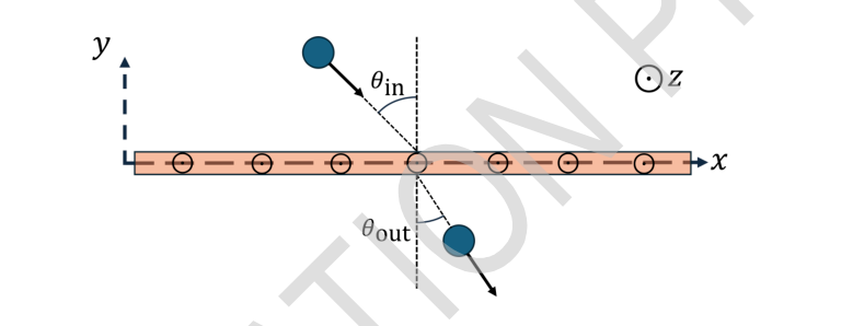
Figure B.3.

Part C. Phase transitions in spin chains (4.3 points)

Next we consider the same chain made of $N$ spins from Part B, except the spin vectors are now restricted to point either up or down along the $z$-axis, so that the spin component along $z$ can be written as $S_{i,z}=s_{i}S$, where $s_i=\pm 1$, see Figure C.1. In addition to the nearest neighbor interactions, we could have an external magnetic field pointing along the $z$-axis so that the total energy of the system is given by

$E=-\tilde{J}{\sum }_i{s}_i{s}_{i+1}-h{\sum }_i{s}_i.$

We assume $\tilde{J}\ge 0$, and $h$ is a constant dependent on the magnetic field. The spin system is at equilibrium with a heat bath at temperature $T$. Ignore the edges of the chain.

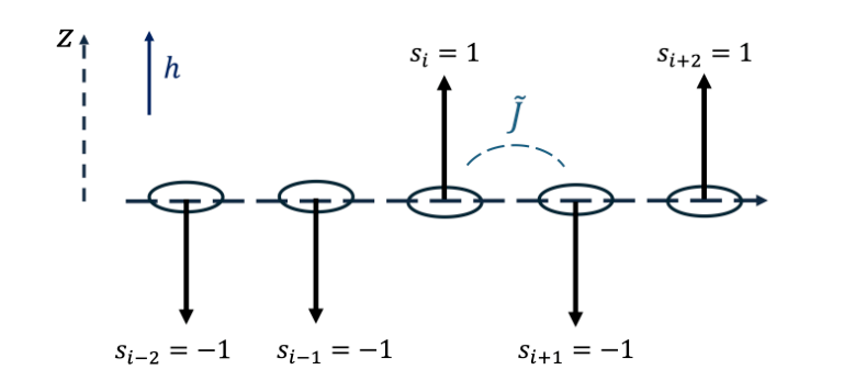
Figure C.1.

C.1 (0.5 pt) Assume first that $\tilde{J}=0$, what is the ratio between the probability to find an arbitrary spin aligned to the magnetic field $p_{\uparrow }$ to being anti-aligned to the magnetic field $p_{\downarrow }$? Express $p_{\uparrow }/p_{\downarrow }$ in terms of $h$, $T$ and fundamental constants.

C.2 (1.0 pt) Find the average polarization of the system $\bar{s}\equiv \frac{1}{N}{\sum }_i{s}_i$ for $N\gg 1$ in terms of $h$, $T$ and fundamental constants. If the magnetic field $h$ can range from $-h_0$ to $h_0$, make a sketch of $\bar{s}$ as a function of $h$ for the cases $h_o\gg k_{B}T$, $h_o\approx k_{B}T$ and $h_o\ll k_{B}T$.

In the remaining questions, we turn off the magnetic field, so $h=0$, and set $\tilde{J}>0$.

C.3 (0.2 pt) What is the energy $E_g$ of the ground state (the lowest energy state)? Express your answer in terms of $\tilde{J}$ and $N$.

Instead of considering the interactions between each spin and its neighbors, we assume that each spin sees an average polarization $\bar{s}$ from its nearest-neighbors.

C.4 (0.2 pt) Approximate the energy of the system as a sum over all spins

$E=-{\tilde{J}}_{\text{eff}}{\sum }_i{s}_i$

and express ${\tilde{J}}_{\text{eff}}$ in terms of $\tilde{J}$ and $\bar{s}$.

C.5 (1.2 pt) Using your result from C.2, find an equation that the average polarization $\bar{s}$ must satisfy. The number of solutions to this equation depends on $T$. Find the critical temperature $T_c$ at which the number of solutions changes. Express your answer in terms of $\tilde{J}$ and fundamental constants.

C.6 (1.0 pt) Find all possible values of $\bar{s}$ when $T<T_c$ and $T_c-T\ll T_c$. Express your answers in terms of $T$ and $T_c$. Sketch all possible values of $\bar{s}$ for the temperature $T$ in the range $0\le T\le 2T_c$.

C.7 (0.2 pt) What magnetic phase of matter does $T>T_c$ correspond to? How about when $T<T_c$? Choose between paramagnetic or ferromagnetic.

Fonte: Testo (PDF) — p.1 Topic: Magnetism, Thermodynamics Metodi: Torque & Angular Momentum Analysis, Wave Equation, Statistical Averaging, Differential Equations Competenze: Physical Reasoning, Mathematical Modeling Objects: Magnetic Dipole, Electron

---

Onde e transizioni di fase nei sistemi di spin (10.0 punti)

Introduzione

Nella fisica classica il momento angolare deriva dal moto di un oggetto attorno a un asse, che si tratti di una trottola, di un pianeta in rotazione o di un elettrone in orbita nell’atomo. Nella fisica quantistica, invece, le particelle fondamentali possiedono una forma intrinseca e quantizzata di momento angolare chiamata spin. Questa proprietà svolge un ruolo cruciale in vari fenomeni fisici, che spaziano dalle proprietà dei materiali, come il magnetismo, alle applicazioni moderne, come il calcolo quantistico.

In questo problema tratteremo lo spin in modo classico, il che porterà ad alcuni risultati qualitativamente corretti. Esplorerai la fisica dei sistemi di spin attraverso le interazioni spin-spin, l’evoluzione in campi magnetici e la fisica statistica, per comprendere l’emergere delle onde di spin e delle transizioni di fase nei magneti.

Informazioni utili:

$\cosh (x)\equiv \frac{e^x+e^{-x}}{2},\sinh (x)\equiv \frac{e^x-e^{-x}}{2},\tanh (x)\equiv \frac{\sinh (x)}{\cosh (x)}\approx x-\frac{1}{3}{x}^3\text{ for }|x|\ll 1$

Il campo magnetico dovuto a un dipolo magnetico di momento $\vec{\mu }$ in una posizione $\vec{r}$ da esso è dato da (${\mu }_0$ è la permeabilità del vuoto):

\vec{B} = \frac{\mu_o}{4\pi}\left( \frac{3(\vec{\mu} \cdot \vec{r})\,\vec{r}}{r^5} - \frac{\vec{\mu}}{r^3} \right) \tag{1}

Parte A. Precessione e interazioni dei dipoli magnetici (1.2 punti)

Si consideri un anello di raggio $R$, massa totale $M$ e carica $Q>0$ distribuita uniformemente. L’anello ruota con velocità angolare $\omega$ attorno a un asse perpendicolare che passa per il suo centro di massa.

A.1 (0.3 pt) È possibile scrivere il momento magnetico $\vec{\mu }$ dell’anello in termini del suo momento angolare $\vec{L}$ come $\vec{\mu }=\gamma \vec{L}$. Trova la costante $\gamma$, detta rapporto giromagnetico, di questo sistema in termini di $Q$ e $M$.

L’anello è posto in un campo magnetico uniforme e debole $\vec{B}=B\hat{z}$, che forma un angolo $\theta$ con $\vec{\omega }$, vedi Figura A.1.

Figura A.1.

A.2 (0.4 pt) Trova la frequenza angolare ${\omega }_L$ della precessione del momento angolare (la cosiddetta frequenza di Larmor) dovuta al campo magnetico esterno in termini di $B$ e $\gamma$. Si prenda come verso positivo quello antiorario rispetto a $+z$.

Ora spegniamo il campo magnetico esterno e poniamo un anello identico a una distanza orizzontale $d\gg R$ dall’anello originale, in modo che il momento magnetico del nuovo anello ${\vec{\mu }}_2$ formi un angolo $\theta$ con ${\vec{\mu }}_1$, vedi Figura A.2.

Figura A.2.

A.3 (0.5 pt) L’energia di interazione magnetica tra i due anelli può essere scritta come $U=J_0{\vec{L}}_1\cdot {\vec{L}}_2$, dove $J_0$ è una costante e ${\vec{L}}_i$ è il momento angolare dell’$i$-esimo anello. Trova $J_0$ in termini di $\gamma$, $d$ e costanti fondamentali.

Parte B. Onde di spin (4.5 punti)

In quanto segue studiamo la dinamica degli spin. Uno spin è una particella con momento angolare intrinseco $\vec{S}$, a cui è associato un momento magnetico $\vec{\mu }$ legato a $\vec{S}$ tramite il rapporto giromagnetico come nella Parte A.1, $\vec{\mu }=\gamma \vec{S}$.

I dipoli magnetici di due spin interagiscono tra loro. Tuttavia questa interazione è trascurabile rispetto a un’altra interazione di origine quantomeccanica, che non è presente nei sistemi classici. È interessante notare che l’energia associata a questa interazione quantistica ha la stessa forma trovata nella Parte A.3, scalando con ${\vec{S}}_1\cdot {\vec{S}}_2$, ma con segno opposto.

Ora consideriamo una catena di spin molto lunga. Le posizioni degli spin sono fisse lungo l’asse $x$, con una distanza $a$ che li separa, vedi Figura B.1. Approssimeremo l’energia totale del sistema considerando solo le interazioni tra primi vicini, in modo che l’energia possa essere scritta come

$E=-J{\sum }_i{\vec{S}}_i\cdot {\vec{S}}_{i+1}$

dove $J>0$ è l’intensità dell’interazione e ${\vec{S}}_i$ è il vettore momento angolare di spin dell’$i$-esimo dipolo, di modulo $S$. I vettori di spin sono liberi di ruotare in tre dimensioni. Si noti che il segno dell’energia è diverso da quello della parte precedente. Questa interazione è puramente quantomeccanica.

Figura B.1.

B.1 (0.3 pt) I termini di energia contenenti ${\vec{S}}_i$ nella somma sopra possono essere visti come l’energia di interazione tra un campo magnetico efficace ${\vec{B}}_{i,\text{eff}}$ e il momento magnetico di ${\vec{S}}_i$. Trova ${\vec{B}}_{i,\text{eff}}$ ed esprimi la tua risposta in termini di $J$, del rapporto giromagnetico $\gamma$ e degli altri spin ${\vec{S}}_j$ (specifica gli indici $j$ in relazione a $i$).

B.2 (0.3 pt) Usando il concetto di campo magnetico efficace, esprimi la velocità di variazione dell’$i$-esimo vettore di spin, $d{\vec{S}}_i/dt$, in termini di $J$, ${\vec{S}}_i$ e degli altri spin ${\vec{S}}_j$ (specifica gli indici $j$ in relazione a $i$).

Per il resto della Parte B, si assuma che il sistema sia fortemente magnetizzato lungo la direzione $z$, così da poter usare le approssimazioni $S_{i,z}\approx S$ e $d{S}_{i,z}/dt\approx 0$ per ogni spin, vedi Figura B.2. In questo regime, l’insieme di equazioni che descrive l’evoluzione temporale degli spin è soddisfatto da una soluzione a onda progressiva per $S_{i,x}$ e $S_{i,y}$ caratterizzata da un vettore d’onda $k$ e da una frequenza angolare $\omega$.

Figura B.2.

B.3 (2.0 pt) Trova la relazione tra $\omega$ e $k$ (nota come relazione di dispersione, $\omega (k)$) per le onde di spin in termini di $J$, $S$ e $a$. Suggerimento: esprimi la posizione dell’$i$-esimo spin come $x=a\cdot i$.

L’onda di spin descritta sopra trasporta energia e quantità di moto. A basse energie, la relazione tra la sua energia e la sua quantità di moto ricorda quella di una particella classica massiva con una massa efficace $m_{\text{eff}}$, un concetto noto come quasiparticella.

B.4 (0.6 pt) Per piccoli $k$ ($k\ll 1/a$), trova la massa efficace $m_{\text{eff}}$ dell’onda di spin. Esprimi la tua risposta in termini di $J$, $S$, $a$ e costanti fondamentali.

Le onde di spin possono essere sondate sperimentalmente mediante scattering anelastico di neutroni. Sebbene i neutroni abbiano carica netta nulla, hanno uno spin finito, che consente loro di interagire con gli altri spin.

B.5 (1.3 pt) Si supponga che inizialmente tutti gli spin nella catena siano orientati lungo la direzione $z$. Un neutrone di bassa energia viaggia nel piano $x$–$y$ formando un angolo di incidenza ${\theta }_{in}$ con la catena e viene diffuso con un angolo ${\theta }_{out}$ come mostrato nella Figura B.3. Assumendo che il neutrone ecciti una singola onda di spin a basso vettore d’onda, trova la massa efficace $m_{\text{eff}}$ dell’onda di spin, in termini di ${\theta }_{in}$, ${\theta }_{out}$ e della massa del neutrone $m_n$. Si assuma che la catena resti in quiete.

Figura B.3.

Parte C. Transizioni di fase nelle catene di spin (4.3 punti)

Consideriamo ora la stessa catena costituita da $N$ spin della Parte B, con la differenza che i vettori di spin sono ora vincolati a puntare verso l’alto o verso il basso lungo l’asse $z$, così che la componente di spin lungo $z$ possa essere scritta come $S_{i,z}=s_{i}S$, dove $s_i=\pm 1$, vedi Figura C.1. Oltre alle interazioni tra primi vicini, potremmo avere un campo magnetico esterno diretto lungo l’asse $z$, così che l’energia totale del sistema sia data da

$E=-\tilde{J}{\sum }_i{s}_i{s}_{i+1}-h{\sum }_i{s}_i.$

Assumiamo $\tilde{J}\ge 0$, e $h$ è una costante che dipende dal campo magnetico. Il sistema di spin è in equilibrio con un bagno termico a temperatura $T$. Si trascurino i bordi della catena.

Figura C.1.

C.1 (0.5 pt) Si assuma dapprima che $\tilde{J}=0$: qual è il rapporto tra la probabilità di trovare uno spin arbitrario allineato al campo magnetico $p_{\uparrow }$ e quella di trovarlo anti-allineato al campo magnetico $p_{\downarrow }$? Esprimi $p_{\uparrow }/p_{\downarrow }$ in termini di $h$, $T$ e costanti fondamentali.

C.2 (1.0 pt) Trova la polarizzazione media del sistema $\bar{s}\equiv \frac{1}{N}{\sum }_i{s}_i$ per $N\gg 1$ in termini di $h$, $T$ e costanti fondamentali. Se il campo magnetico $h$ può variare da $-h_0$ a $h_0$, traccia uno schizzo di $\bar{s}$ in funzione di $h$ per i casi $h_o\gg k_{B}T$, $h_o\approx k_{B}T$ e $h_o\ll k_{B}T$.

Nelle domande rimanenti spegniamo il campo magnetico, quindi $h=0$, e poniamo $\tilde{J}>0$.

C.3 (0.2 pt) Qual è l’energia $E_g$ dello stato fondamentale (lo stato di energia più bassa)? Esprimi la tua risposta in termini di $\tilde{J}$ e $N$.

Invece di considerare le interazioni tra ciascuno spin e i suoi vicini, assumiamo che ogni spin veda una polarizzazione media $\bar{s}$ dovuta ai suoi primi vicini.

C.4 (0.2 pt) Approssima l’energia del sistema come una somma su tutti gli spin

$E=-{\tilde{J}}_{\text{eff}}{\sum }_i{s}_i$

ed esprimi ${\tilde{J}}_{\text{eff}}$ in termini di $\tilde{J}$ e $\bar{s}$.

C.5 (1.2 pt) Usando il risultato del punto C.2, trova un’equazione che la polarizzazione media $\bar{s}$ deve soddisfare. Il numero di soluzioni di questa equazione dipende da $T$. Trova la temperatura critica $T_c$ alla quale il numero di soluzioni cambia. Esprimi la tua risposta in termini di $\tilde{J}$ e costanti fondamentali.

C.6 (1.0 pt) Trova tutti i possibili valori di $\bar{s}$ quando $T<T_c$ e $T_c-T\ll T_c$. Esprimi le tue risposte in termini di $T$ e $T_c$. Traccia tutti i possibili valori di $\bar{s}$ per la temperatura $T$ nell’intervallo $0\le T\le 2T_c$.

C.7 (0.2 pt) A quale fase magnetica della materia corrisponde $T>T_c$? E quando $T<T_c$? Scegli tra paramagnetica e ferromagnetica.

Fonte: Testo (PDF) — p.1 Topic: Magnetism, Thermodynamics Metodi: Torque & Angular Momentum Analysis, Wave Equation, Statistical Averaging, Differential Equations Competenze: Physical Reasoning, Mathematical Modeling Objects: Magnetic Dipole, Electron

---

Atmospheric Physics (10.0 points)

The Earth’s atmosphere is a complex physical system, and predicting its behavior is crucial for environmental and meteorological purposes. However, even the best theoretical models run on modern computers are insufficient to make precise predictions. In this problem, we will attempt to understand some of the basic atmospheric phenomena based on simple models. You might need the following constants: the mean solar power per unit area at Earth, the total solar irradiance $F_s=1370{\text{W/m}}^2$, molar mass of water ${\mu }_{{\text{H}}_2\text{O}}\approx 18\text{g/mol}$ and average molar mass of air ${\mu }_{\text{air}}\approx 29\text{g/mol}$, The Stefan-Boltzmann constant $\sigma =5.67\times 10^{-8}{\text{W/(m}}^2{\text{K}}^4)$. All gases in this problem can be treated as ideal gases. Assume that all air molecules have $5$ degrees of freedom. You may need the following integral:

${\int }_{-\infty }^{\infty }{e}^{-a{x}^2/2}dx=\sqrt{\frac{2\pi }{a}},a>0.$

Part A. Surface Temperature of the Earth (1.2 points)

In this section, we study the effect of the atmosphere on the Earth surface’s temperature. Assume that Earth and its atmosphere have an albedo $a=0.3$ for solar radiation, which is the reflected fraction of the total incident radiation. You may use this value in all parts of this problem. In addition, assume the Earth radiates as a black body.

A.1 (0.2 pt) Express the average net solar power received by the Earth and atmosphere system $P_0$ in terms of $F_s$, $a$ and $R_E$, the radius of the Earth.

A.2 (0.3 pt) Estimate the temperature of the Earth’s surface $T_{g0}$ assuming that it is at a steady state. Ignore the atmosphere.

Your answer for A.2 should be lower than what you would expect. We now consider adding a thin atmospheric layer at temperature $T_a$, see Figure A.1. The atmospheric layer transmits a net fraction $t_{sw}$ of the incident solar radiation and a net fraction $t_{lw}$ of the Earth’s thermal radiation. Otherwise, you may treat the atmosphere as a black body.

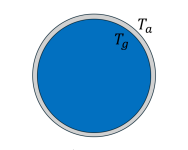
Figure A.1

A.3 (0.7 pt) Assuming the system is in a steady state, calculate $T_g$, the temperature of the ground. Use $t_{sw}=0.9$ and $t_{lw}=0.2$.

Part B. The absorption spectrum of atmospheric gases (1.8 points)

The infrared radiation emitted by Earth has low energy, incapable of exciting electrons within the molecules, but it has the ability to excite the vibrational and rotational modes of the molecules.

B.1 (0.5 pt) Consider a simple diatomic molecule modeled as two point masses $m_A$ and $m_B$ connected by a spring with spring constant $k$. What is the angular frequency of vibrations ${\omega }_d$?

B.2 (0.2 pt) Quantum mechanics dictates that vibrational excitations due to absorbing a photon can only raise the quantum energy level by one. What is the energy of the photon $E_p$ that can excite the vibration in B.1? Neglect recoil effects.

Quantum mechanics forbids the vibrational modes of symmetric diatomic molecules, such as nitrogen and oxygen (the most abundant gasses in the Earth’s atmosphere) to be excited by light. This explains why ${\text{N}}_2$ and ${\text{O}}_2$ do not contribute to the green house effect. In general, the absorption of light by molecules is governed by the allowed energy transitions in them. However, the energy of the light absorbed does not have to exactly match the energy gap in the molecule. Suppose that a molecule at rest has a spectral line (an allowed transition) at frequency $f_0$.

B.3 (0.2 pt) What is the shift in the spectral line $f-f_0$ if the molecule is moving with velocity $v$ towards the emitter such that $|v|\ll c$, where $c$ is the speed of light.

For a gas at temperature $T$, the velocity of its molecules is distributed according to Maxwell’s distribution. For a molecule of mass $m$, the probability to find a molecule’s velocity along one dimension to be between $v$ and $v+dv$ is $p_1(v)dv$, where $p_1(v)$ is a probability distribution function given by

$p_1(v)=C\exp \left(-\frac{m{v}^2}{2k_{B}T}\right)$

$C$ is a normalization constant ensuring the probabilities add up to one, and $k_B$ is the Boltzmann constant.

B.4 (0.2 pt) Find the normalization constant $C$, assuming that the velocity $v$ could range from $-\infty$ to $\infty$.

B.5 (0.3 pt) Find the probability distribution function $p_2(f)$ to find a molecule with a spectral line $f_0$ shifted to $f$ due to thermal motion, up to a normalization factor, in terms of $f$, $f_0$, $T$, $m$ and fundamental constants.

B.6 (0.4 pt) Sketch $p_2(f)$ as a function of $f-f_0$, and determine the shift $f^{\star }-f_0$ at which $p_2(f^{\star })$ is a fraction $1/e$ of its peak value, where $e$ is the natural number.

Part C. Stability of air in the atmosphere (2.7 points)

Consider a small cylindrical mass of air at height $z$ above the ground. The pressure and mass density of air at that height are $p(z)$ and $\rho (z)$, respectively, see Figure C.1. Assume a uniform downward gravitational field $g$ and that the pressure on the Earth’s surface is $p_o$.

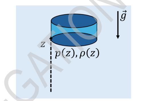
Figure C.1

C.1 (0.3 pt) Assuming that the small air mass is at hydrostatic equilibrium, derive an expression of the rate of change of pressure with respect to height, $dp/dz$ in terms of $g$ and $\rho (z)$.

C.2 (0.2 pt) Express $dp/dz$ in terms of ${\mu }_{\text{air}}$, $g$, $p(z)$ and $T(z)$, the temperature at height $z$ and fundamental constants.

C.3 (0.2 pt) Assuming an isothermal atmosphere, $T(z)=T$, find an expression for $p(z)$ in terms of $z$, ${\mu }_{\text{air}}$, $g$, $p_o$, $T$ and fundamental constants.

In a real atmosphere, the temperature is not constant but changes with height. The rate of decrease of temperature with height $\Gamma (z)=-dT/dz$ is called the lapse rate. Consider a small mass of air rising adiabatically in the atmosphere such that it remains at mechanical equilibrium with its surrounding.

C.4 (0.6 pt) For the adiabatically rising air mass, find the adiabatic lapse rate ${\Gamma }_a$ in terms of $c_p$, the molar specific heat at constant pressure, ${\mu }_{\text{air}}$ and $g$.

To analyze the stability of an atmosphere, we imagine starting from an equilibrium state, and then perturbing a small mass of air and analyze its response. Consider a small air mass initially in equilibrium with the surrounding air at height $z$ and temperature $T$. It is then adiabatically displaced vertically by a displacement $\delta z_0$. Assume that throughout the motion, the air parcel always has the same pressure as the surrounding air at the same height. The surrounding atmosphere is unaltered and has a different lapse rate $\Gamma$. Neglect viscosity.

C.5 (1.4 pt) Find the equation of motion for $\delta z$, the instantaneous vertical displacement. Under what condition is the equilibrium at $z$ stable? What is the angular frequency $\omega$ of small oscillation? Express your answers in terms of $T$, $\Gamma$, $g$, ${\mu }_{\text{air}}$ and $c_p$.

Part D. Moisture (2.7 points)

Even though water constitutes a small portion of the atmosphere, it has a significant role in climate science. It is responsible for precipitation, and it is the most significant greenhouse gas. The phase of water depends on what temperature and pressure the water system is at, depicted on a $p$–$T$ phase diagram, see Figure D.1. When the pressure and temperature lie on the coexistence curve, both liquid and vapor water can be present in the system. The slope of the coexistence curve is given by the Clausius-Clapeyron equation:

$\frac{d{p}_s}{dT}=\frac{\Delta S}{\Delta V}$

where $p_s$ is the saturation pressure, the pressure at the phase transition, $\Delta S$ and $\Delta V$ are the changes in entropy and volume across the phase transitions, respectively. Treat water vapor as an ideal gas.

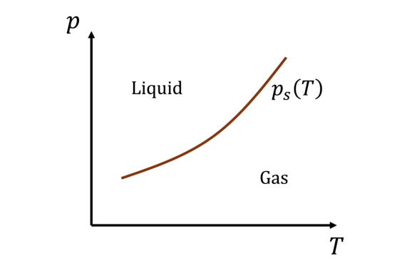
Figure D.1

D.1 (0.5 pt) Express $d{p}_s/dT$ for the water liquid-vapor coexistence curve in terms of the water latent heat of evaporation $L$, ${\mu }_{{\text{H}}_2\text{O}}$, $p_s$, $T$ and fundamental constants.

D.2 (0.2 pt) If for some reference temperature $T_o$, $p_s=p_{so}$, find an expression for $p_s(T)$ in terms of $p_{so}$, ${\mu }_{{\text{H}}_2\text{O}}$, $L$, $T$, $T_o$ and fundamental constants.

Now we consider a ‘moist’ air mass that rises adiabatically starting from a temperature $T_i$. The mass mixing ratio of water vapor (the mass of water vapor relative to the total mass) is $\varphi$. Take the air mass to have a specific molar heat at constant pressure $c_p$. The universal gas constant is $R=8.31\text{J/(mol K)}$.

D.3 (2.0 pt) Assuming that the air mass starts at $T_i=17.0^{\circ }\text{C}$ and $p_i=10^5\text{Pa}$. Find the temperature $T_l$ at which liquid water starts forming in it if $\varphi =10^{-2}$. Assume that the water content in the air mass stays constant during the rise. Use $L=2460\text{kJ/kg}$ and $p_{so}=1.94\times 10^3\text{Pa}$ at $T_i=17.0^{\circ }\text{C}$.

Part E. Sun halo (1.6 points)

Under suitable atmospheric conditions, a bright ring appears around the Sun which is called a halo. Halos are caused by ice crystals present in the upper troposphere. One interesting feature about halos is that they always appear at a specific angle relative to the direction of the Sun.

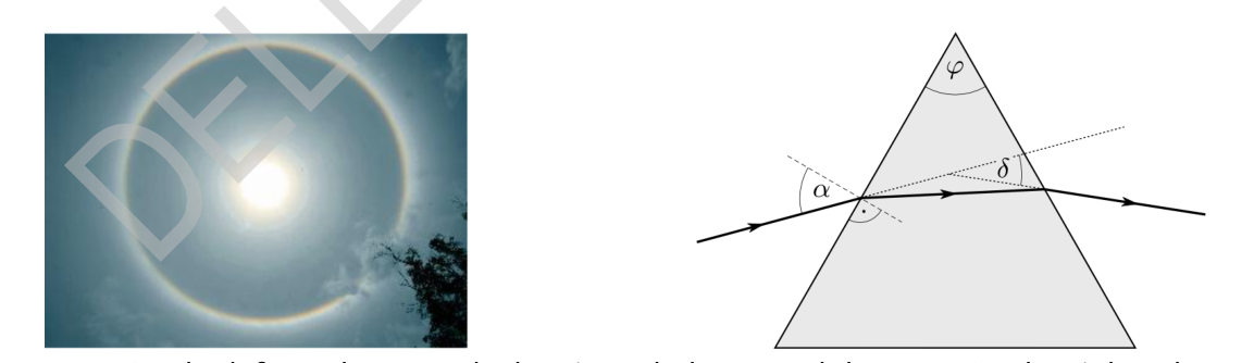
Figure E.1. On the left: A photograph showing a halo around the Sun. On the right: The path of a light ray passing through the prism.

E.1 (0.8 pt) Consider a simple prism with an apex angle of $\phi$ and direct a light ray onto it at an incidence angle $\alpha$, as shown in Figure E.1. Let the refractive index of the prism be $n$. Express the angle of deviation $\delta$ of the light ray after passing through the prism in terms of $\alpha$, $n$ and $\phi$.

The most common type of halo forms when tiny ice crystals take the shape of regular hexagonal prisms. Light from the Sun falls onto randomly oriented ice crystals drifting in the atmosphere and scatters into various directions. However, in certain specific directions, the intensity of the refracted light is maximal, and this determines the angle at which the bright ring appears.

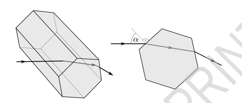
Figure E.2.

Consider a hexagonal ice prism whose six-fold symmetry axis is perpendicular to the direction of the Sun’s rays. Investigate a light ray that refracts through two rectangular faces of the prism indicated in Figure E.2. Due to the random orientation of the ice crystals, the light strikes the crystal faces at varying incidence angles $\alpha$.

E.2 (0.6 pt) Plot on the answer sheet how the deviation angle $\delta$ of the examined light ray depends on the incidence angle $\alpha$ within the interval $[20^{\circ },70^{\circ }]$ in $5^{\circ }$ increments. The refractive index of ice is $n=1.31$.

E.3 (0.2 pt) Using the graph from the previous part, determine at what angle the halo appears the brightest relative to the direction of the Sun.

Fonte: Testo (PDF) — p.1 Topic: Thermodynamics, Earth & Environmental Science Metodi: First Law of Thermodynamics, Hydrostatic Equilibrium, Kinetic Theory of Gases, Snell’s Law Competenze: Physical Reasoning, Estimation & Approximation Objects: Planet, Star, Gas, Spring, Prism

Fisica dell’atmosfera (10.0 punti)

L’atmosfera terrestre è un sistema fisico complesso e prevederne il comportamento è cruciale per scopi ambientali e meteorologici. Tuttavia, persino i migliori modelli teorici eseguiti su computer moderni sono insufficienti per fare previsioni precise. In questo problema cercheremo di comprendere alcuni dei fenomeni atmosferici fondamentali sulla base di modelli semplici. Potresti aver bisogno delle seguenti costanti: la potenza solare media per unità di area sulla Terra, l’irradianza solare totale $F_s=1370{\text{W/m}}^2$, la massa molare dell’acqua ${\mu }_{{\text{H}}_2\text{O}}\approx 18\text{g/mol}$ e la massa molare media dell’aria ${\mu }_{\text{air}}\approx 29\text{g/mol}$, la costante di Stefan-Boltzmann $\sigma =5.67\times 10^{-8}{\text{W/(m}}^2{\text{K}}^4)$. Tutti i gas in questo problema possono essere trattati come gas ideali. Si assuma che tutte le molecole d’aria abbiano $5$ gradi di libertà. Potresti aver bisogno del seguente integrale:

${\int }_{-\infty }^{\infty }{e}^{-a{x}^2/2}dx=\sqrt{\frac{2\pi }{a}},a>0.$

Parte A. Temperatura superficiale della Terra (1.2 punti)

In questa sezione studiamo l’effetto dell’atmosfera sulla temperatura della superficie terrestre. Si assuma che la Terra e la sua atmosfera abbiano un’albedo $a=0.3$ per la radiazione solare, cioè la frazione riflessa della radiazione incidente totale. Puoi usare questo valore in tutte le parti di questo problema. Inoltre, si assuma che la Terra irradi come un corpo nero.

A.1 (0.2 pt) Esprimi la potenza solare netta media ricevuta dal sistema Terra-atmosfera $P_0$ in termini di $F_s$, $a$ e $R_E$, il raggio della Terra.

A.2 (0.3 pt) Stima la temperatura della superficie terrestre $T_{g0}$ assumendo che sia in stato stazionario. Trascura l’atmosfera.

La tua risposta per A.2 dovrebbe essere più bassa di quanto ti aspetteresti. Consideriamo ora di aggiungere un sottile strato atmosferico a temperatura $T_a$, vedi Figura A.1. Lo strato atmosferico trasmette una frazione netta $t_{sw}$ della radiazione solare incidente e una frazione netta $t_{lw}$ della radiazione termica della Terra. Per il resto, puoi trattare l’atmosfera come un corpo nero.

Figura A.1

A.3 (0.7 pt) Assumendo che il sistema sia in stato stazionario, calcola $T_g$, la temperatura del suolo. Usa $t_{sw}=0.9$ e $t_{lw}=0.2$.

Parte B. Lo spettro di assorbimento dei gas atmosferici (1.8 punti)

La radiazione infrarossa emessa dalla Terra ha bassa energia, incapace di eccitare gli elettroni all’interno delle molecole, ma ha la capacità di eccitare i modi vibrazionali e rotazionali delle molecole.

B.1 (0.5 pt) Si consideri una semplice molecola biatomica modellizzata come due masse puntiformi $m_A$ e $m_B$ collegate da una molla con costante elastica $k$. Qual è la frequenza angolare delle vibrazioni ${\omega }_d$?

B.2 (0.2 pt) La meccanica quantistica impone che le eccitazioni vibrazionali dovute all’assorbimento di un fotone possano innalzare il livello energetico quantico solo di uno. Qual è l’energia del fotone $E_p$ che può eccitare la vibrazione in B.1? Trascura gli effetti di rinculo.

La meccanica quantistica proibisce che i modi vibrazionali delle molecole biatomiche simmetriche, come l’azoto e l’ossigeno (i gas più abbondanti nell’atmosfera terrestre), siano eccitati dalla luce. Ciò spiega perché ${\text{N}}_2$ e ${\text{O}}_2$ non contribuiscono all’effetto serra. In generale, l’assorbimento della luce da parte delle molecole è governato dalle transizioni energetiche permesse in esse. Tuttavia, l’energia della luce assorbita non deve necessariamente coincidere esattamente con il salto energetico nella molecola. Si supponga che una molecola in quiete abbia una riga spettrale (una transizione permessa) alla frequenza $f_0$.

B.3 (0.2 pt) Qual è lo spostamento della riga spettrale $f-f_0$ se la molecola si muove con velocità $v$ verso l’emettitore tale che $|v|\ll c$, dove $c$ è la velocità della luce.

Per un gas a temperatura $T$, la velocità delle sue molecole è distribuita secondo la distribuzione di Maxwell. Per una molecola di massa $m$, la probabilità che la velocità di una molecola lungo una dimensione sia compresa tra $v$ e $v+dv$ è $p_1(v)dv$, dove $p_1(v)$ è una funzione di distribuzione di probabilità data da

$p_1(v)=C\exp \left(-\frac{m{v}^2}{2k_{B}T}\right)$

$C$ è una costante di normalizzazione che garantisce che le probabilità sommino a uno, e $k_B$ è la costante di Boltzmann.

B.4 (0.2 pt) Trova la costante di normalizzazione $C$, assumendo che la velocità $v$ possa variare da $-\infty$ a $\infty$.

B.5 (0.3 pt) Trova la funzione di distribuzione di probabilità $p_2(f)$ di trovare una molecola con una riga spettrale $f_0$ spostata a $f$ a causa del moto termico, a meno di un fattore di normalizzazione, in termini di $f$, $f_0$, $T$, $m$ e costanti fondamentali.

B.6 (0.4 pt) Traccia $p_2(f)$ in funzione di $f-f_0$, e determina lo spostamento $f^{\star }-f_0$ per il quale $p_2(f^{\star })$ è una frazione $1/e$ del suo valore di picco, dove $e$ è il numero di Nepero.

Parte C. Stabilità dell’aria nell’atmosfera (2.7 punti)

Si consideri una piccola massa d’aria cilindrica ad altezza $z$ sopra il suolo. La pressione e la densità di massa dell’aria a quell’altezza sono rispettivamente $p(z)$ e $\rho (z)$, vedi Figura C.1. Si assuma un campo gravitazionale uniforme diretto verso il basso $g$ e che la pressione sulla superficie terrestre sia $p_o$.

Figura C.1

C.1 (0.3 pt) Assumendo che la piccola massa d’aria sia in equilibrio idrostatico, ricava un’espressione della variazione della pressione rispetto all’altezza, $dp/dz$ in termini di $g$ e $\rho (z)$.

C.2 (0.2 pt) Esprimi $dp/dz$ in termini di ${\mu }_{\text{air}}$, $g$, $p(z)$ e $T(z)$, la temperatura all’altezza $z$, e costanti fondamentali.

C.3 (0.2 pt) Assumendo un’atmosfera isoterma, $T(z)=T$, trova un’espressione per $p(z)$ in termini di $z$, ${\mu }_{\text{air}}$, $g$, $p_o$, $T$ e costanti fondamentali.

In un’atmosfera reale la temperatura non è costante, ma varia con l’altezza. Il tasso di diminuzione della temperatura con l’altezza $\Gamma (z)=-dT/dz$ è detto gradiente termico verticale (lapse rate). Si consideri una piccola massa d’aria che sale adiabaticamente nell’atmosfera rimanendo in equilibrio meccanico con l’ambiente circostante.

C.4 (0.6 pt) Per la massa d’aria che sale adiabaticamente, trova il gradiente adiabatico ${\Gamma }_a$ in termini di $c_p$, il calore specifico molare a pressione costante, ${\mu }_{\text{air}}$ e $g$.

Per analizzare la stabilità di un’atmosfera, immaginiamo di partire da uno stato di equilibrio, quindi perturbiamo una piccola massa d’aria e ne analizziamo la risposta. Si consideri una piccola massa d’aria inizialmente in equilibrio con l’aria circostante ad altezza $z$ e temperatura $T$. Essa viene poi spostata adiabaticamente in verticale di uno spostamento $\delta z_0$. Si assuma che durante tutto il moto la particella d’aria abbia sempre la stessa pressione dell’aria circostante alla stessa altezza. L’atmosfera circostante è inalterata e ha un diverso gradiente $\Gamma$. Trascura la viscosità.

C.5 (1.4 pt) Trova l’equazione del moto per $\delta z$, lo spostamento verticale istantaneo. Sotto quale condizione l’equilibrio in $z$ è stabile? Qual è la frequenza angolare $\omega$ delle piccole oscillazioni? Esprimi le tue risposte in termini di $T$, $\Gamma$, $g$, ${\mu }_{\text{air}}$ e $c_p$.

Parte D. Umidità (2.7 punti)

Sebbene l’acqua costituisca una piccola porzione dell’atmosfera, ha un ruolo significativo nella scienza del clima. È responsabile delle precipitazioni ed è il gas serra più importante. La fase dell’acqua dipende dalla temperatura e dalla pressione a cui si trova il sistema acqua, rappresentate su un diagramma di fase $p$–$T$, vedi Figura D.1. Quando la pressione e la temperatura giacciono sulla curva di coesistenza, nel sistema possono essere presenti sia acqua liquida sia vapore. La pendenza della curva di coesistenza è data dall’equazione di Clausius-Clapeyron:

$\frac{d{p}_s}{dT}=\frac{\Delta S}{\Delta V}$

dove $p_s$ è la pressione di saturazione, la pressione alla transizione di fase, $\Delta S$ e $\Delta V$ sono rispettivamente le variazioni di entropia e di volume attraverso le transizioni di fase. Tratta il vapore acqueo come un gas ideale.

Figura D.1

D.1 (0.5 pt) Esprimi $d{p}_s/dT$ per la curva di coesistenza liquido-vapore dell’acqua in termini del calore latente di evaporazione dell’acqua $L$, ${\mu }_{{\text{H}}_2\text{O}}$, $p_s$, $T$ e costanti fondamentali.

D.2 (0.2 pt) Se per una certa temperatura di riferimento $T_o$ si ha $p_s=p_{so}$, trova un’espressione per $p_s(T)$ in termini di $p_{so}$, ${\mu }_{{\text{H}}_2\text{O}}$, $L$, $T$, $T_o$ e costanti fondamentali.

Consideriamo ora una massa d’aria ‘umida’ che sale adiabaticamente partendo da una temperatura $T_i$. Il rapporto di mescolamento in massa del vapore acqueo (la massa di vapore acqueo rispetto alla massa totale) è $\varphi$. Si assuma che la massa d’aria abbia un calore specifico molare a pressione costante $c_p$. La costante universale dei gas è $R=8.31\text{J/(mol K)}$.

D.3 (2.0 pt) Assumendo che la massa d’aria parta da $T_i=17.0^{\circ }\text{C}$ e $p_i=10^5\text{Pa}$. Trova la temperatura $T_l$ alla quale l’acqua liquida inizia a formarsi in essa se $\varphi =10^{-2}$. Si assuma che il contenuto d’acqua nella massa d’aria resti costante durante la salita. Usa $L=2460\text{kJ/kg}$ e $p_{so}=1.94\times 10^3\text{Pa}$ a $T_i=17.0^{\circ }\text{C}$.

Parte E. Alone solare (1.6 punti)

In condizioni atmosferiche opportune, attorno al Sole appare un anello luminoso chiamato alone. Gli aloni sono causati dai cristalli di ghiaccio presenti nell’alta troposfera. Una caratteristica interessante degli aloni è che appaiono sempre a uno specifico angolo rispetto alla direzione del Sole.

Figura E.1. A sinistra: Una fotografia che mostra un alone attorno al Sole. A destra: Il cammino di un raggio di luce che attraversa il prisma.

E.1 (0.8 pt) Si consideri un semplice prisma con angolo al vertice $\phi$ e si diriga su di esso un raggio di luce con angolo di incidenza $\alpha$, come mostrato nella Figura E.1. Sia $n$ l’indice di rifrazione del prisma. Esprimi l’angolo di deviazione $\delta$ del raggio di luce dopo l’attraversamento del prisma in termini di $\alpha$, $n$ e $\phi$.

Il tipo più comune di alone si forma quando minuscoli cristalli di ghiaccio assumono la forma di prismi esagonali regolari. La luce del Sole cade su cristalli di ghiaccio orientati casualmente che vagano nell’atmosfera e viene diffusa in varie direzioni. Tuttavia, in certe direzioni specifiche l’intensità della luce rifratta è massima, e ciò determina l’angolo a cui appare l’anello luminoso.

Figura E.2.

Si consideri un prisma esagonale di ghiaccio il cui asse di simmetria di ordine sei è perpendicolare alla direzione dei raggi del Sole. Studia un raggio di luce che si rifrange attraverso due facce rettangolari del prisma indicate nella Figura E.2. A causa dell’orientamento casuale dei cristalli di ghiaccio, la luce colpisce le facce del cristallo con angoli di incidenza $\alpha$ variabili.

E.2 (0.6 pt) Traccia sul foglio delle risposte come l’angolo di deviazione $\delta$ del raggio di luce esaminato dipende dall’angolo di incidenza $\alpha$ nell’intervallo $[20^{\circ },70^{\circ }]$ a passi di $5^{\circ }$. L’indice di rifrazione del ghiaccio è $n=1.31$.

E.3 (0.2 pt) Usando il grafico della parte precedente, determina a quale angolo l’alone appare più luminoso rispetto alla direzione del Sole.

Fonte: Testo (PDF) — p.1 Topic: Thermodynamics, Earth & Environmental Science Metodi: First Law of Thermodynamics, Hydrostatic Equilibrium, Kinetic Theory of Gases, Snell’s Law Competenze: Physical Reasoning, Estimation & Approximation Objects: Planet, Star, Gas, Spring, Prism