OII na Sperimentale

Wiedemann-Franz law – Appendix, Part A: regime quasi-stazionario e correzione della conducibilità termica

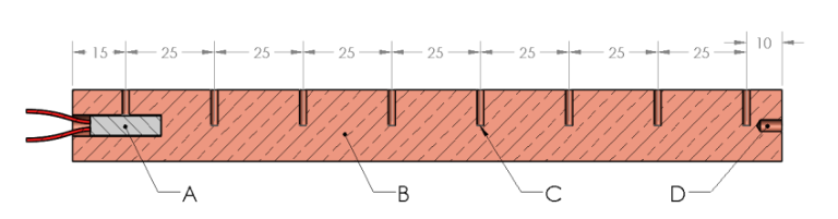
Si usa un semplice modello per analizzare il trasporto di calore attraverso la barretta. Un riscaldatore fornisce potenza $P_0$ a un’estremità. In ogni punto vale:

$P_T=-\kappa A\frac{\partial T}{\partial x}$

dove $P_T$ è la corrente di calore nel punto $x$. Idealmente $P_T$ dovrebbe essere costante lungo la barretta. Tuttavia, due meccanismi modificano questo comportamento: (a) la potenza dissipata per variare la temperatura del materiale; (b) la perdita di potenza verso l’ambiente. L’equazione completa è:

$\frac{\partial P}{\partial x}=-\rho c_{p}A\frac{\partial T}{\partial t}-K(T-T_0)$

dove $c_p$ è il calore specifico, $\rho$ la densità, $K$ il parametro di perdita termica radiale per unità di lunghezza, e $T_0$ la temperatura ambiente.

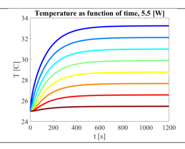
La scala temporale del processo di riscaldamento è 2 minuti e 30 secondi, per cui si raggiunge il 95% del valore finale dopo 7 minuti e 30 secondi (come mostrato nel grafico in alto). Tuttavia, questo è valido solo per un sistema ideale. Nel sistema reale, il collegamento al serbatoio termico non è ideale e vi sono perdite radiali. Il sistema è modellizzato come una barretta collegata tramite resistenza termica a una corta barretta di alluminio (che rappresenta la pentola e il dissipatore termico), a sua volta connessa a un serbatoio d’acqua.

Part A – Sistema ideale e correzione al prim’ordine

Per un sistema ideale (barretta connessa solo a un serbatoio ideale), si ottiene un gradiente di temperatura costante:

$\frac{\Delta T}{\Delta x}=-\frac{P}{\kappa A}\Rightarrow \kappa =\frac{P}{A\cdot \text{Slope}}$

che fornisce $\kappa =385W/(\mathrm{m}\cdot \mathrm{K})$.

I meccanismi di perdita influenzano il flusso di calore ma esiste sempre una relazione locale tra il gradiente di temperatura e il calore locale. Il gradiente vicino al riscaldatore è determinato dalla potenza $P$, mentre il gradiente vicino al serbatoio è determinato da $P-P_{\text{loss}}$. La correzione al prim’ordine alla pendenza è:

$\frac{\Delta T_1/\Delta x_1}{\Delta T_2/\Delta x_2}=\frac{P-P_{\text{absorb}}-P_{\text{loss}}}{P}=1-\frac{c_{p}m}{P}\frac{\partial T}{\partial t}-\frac{P_{\text{loss}}}{P}$

Con queste due correzioni l’accuratezza migliora a meno dell’1%, rispetto all’8% senza correzione.

Temperatura vs tempo verso regime stazionario

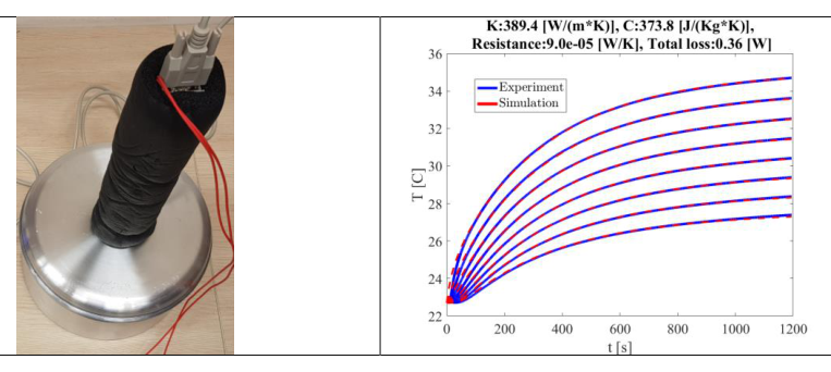
Simulazione confrontata con dati misurati

Accuratezza della correzione al prim’ordine

Topic: Thermodynamics, Electromagnetic Induction Metodi: First Law of Thermodynamics, Differential Equations, Physical Modeling Competenze: Mathematical Modeling, Physical Reasoning Objects: Rod Fonte: Testo (PDF) — p.1 Soluzione: Soluzioni (PDF)

Wiedemann-Franz law Appendix, Part A: quasi-stationary regime and correction of thermal conductivity

A simple model is used to analyze the heat transfer through the barrel. A heater provides $P_0$ power to one end. In each case:

$P_T=-\kappa A\frac{\partial T}{\partial x}$

where $P_T$ is the heat current in $x$. Ideally $P_T$ should be constant along the bar. However, two mechanisms change this behaviour: (a) the power dissipated to change the temperature of the material; (b) the loss of power to the environment. The full equation is:

$\frac{\partial P}{\partial x}=-\rho c_{p}A\frac{\partial T}{\partial t}-K(T-T_0)$

where $c_p$ is the specific heat, $\rho$ the density, $K$ the radial thermal loss parameter per unit length, and $T_0$ the ambient temperature.

The heating time scale is 2 minutes and 30 seconds, so 95% of the final value is reached after 7 minutes and 30 seconds (as shown in the graph above). However, this is only valid for an ideal system. In the real system, the connection to the heat tank is not ideal and there are radial leaks. The system is modelled as a bar connected by thermal resistance to a short aluminium bar (representing the pot and the heat dissipator), which in turn is connected to a water tank.

Part A Ideal system and first order correction

For an ideal system (barrel connected only to an ideal tank), a constant temperature gradient is obtained:

$\frac{\Delta T}{\Delta x}=-\frac{P}{\kappa A}\Rightarrow \kappa =\frac{P}{A\cdot \text{Slope}}$

which provides $\kappa =385W/(\mathrm{m}\cdot \mathrm{K})$.

The loss mechanisms affect the heat flow but there is always a local relationship between the temperature gradient and the local heat. The gradient near the heater is determined by $P$ power, while the gradient near the tank is determined by $P-P_{\text{loss}}$. The first-order correction of slope is:

$\frac{\Delta T_1/\Delta x_1}{\Delta T_2/\Delta x_2}=\frac{P-P_{\text{absorb}}-P_{\text{loss}}}{P}=1-\frac{c_{p}m}{P}\frac{\partial T}{\partial t}-\frac{P_{\text{loss}}}{P}$

With these two corrections, accuracy improves to less than 1%, compared to 8% without correction.

The following table shows the temperature and time to steady state:

Simulation compared with measured data

Accuracy of the first order correction

Topic: Thermodynamics, Electromagnetic Induction Metodi: First Law of Thermodynamics, Differential Equations, Physical Modeling Competenze: Mathematical Modeling, Physical Reasoning Objects: Rod Fonte: Testo (PDF) — p.1 Soluzione: Soluzioni (PDF)

Wiedemann-Franz law – Appendix, Part B: ciclo raffreddamento–riscaldamento–raffreddamento

Lo scopo di questa sezione è ottenere la perdita di calore $P_{\text{loss}}$ e la capacità termica $C=c_{p}m$ della barretta, al fine di correggere l’errore dell’8% del risultato della Parte A. Si disconnette la barretta dal serbatoio termico, si isola l’estremità libera e si riscalda fino a circa la temperatura della sezione precedente.

Si esegue un ciclo raffreddamento–riscaldamento–raffreddamento per ottenere $c_{p}m$ e $P_{\text{loss}}$.

Metodo (a) – basato sulla pendenza di $T(t)$:

Durante il raffreddamento: ${\frac{\partial T_{\text{av}}}{\partial t}|}_{\text{Cooling}}=-\frac{P_{\text{loss}}}{c_{p}m}$

Durante il riscaldamento: ${\frac{\partial T_{\text{av}}}{\partial t}|}_{\text{Heating}}-{\frac{\partial T_{\text{av}}}{\partial t}|}_{\text{Cooling}}=\frac{P_{\text{in}}}{c_{p}m}$

permettendo di ricavare $c_p\cdot m$.

Metodo (b) – basato sull’energia totale:

Il calore totale immesso durante l’intervallo di riscaldamento, $P_{\text{in}}\cdot \Delta t_{\text{Heating}}$, è legato a $\Delta T_{\text{Heating}}$ (lo spostamento verticale tra le rette di raffreddamento $T(t)$ prima e dopo il riscaldamento) dalla relazione:

$P_{\text{in}}\Delta t_{\text{Heating}}=c_{p}m\Delta T_{\text{Heating}}$

Entrambi i metodi riproducono la conducibilità termica entro l’1%, con $c_p=386J/(\mathrm{kg}\cdot \mathrm{K})$.

La perdita di calore totale è: $P_{\text{loss}}=-c_p\cdot m\cdot {\frac{\partial T_{\text{av}}}{\partial t}|}_{\text{Cooling}}=0.34J/s$

Nota: un contributo significativo alla capacità termica proviene dall’isolamento e da altri componenti del sistema; si deve pertanto usare una massa efficace maggiore della massa reale. Questo è rilevante solo per ottenere il corretto $c_p$, mentre per il resto dell’esperimento si usa solo il prodotto $c_{p}m$.

A seconda del metodo, il risultato di $C$ può deviare del 5%, producendo un errore trascurabile di meno dello 0.5% nel risultato della conducibilità termica.

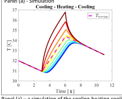Simulazione ciclo raffreddamento-riscaldamento-raffreddamento

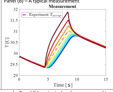Misurazione tipica del ciclo con termometri

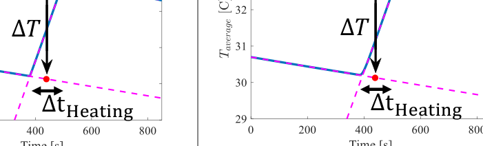Grafico T(t) con ΔT e Δt_Heating indicati

Topic: Thermodynamics Metodi: First Law of Thermodynamics, Experimental Data Analysis, Physical Modeling Competenze: Experimental Data Analysis, Graph Linearization Objects: Rod Fonte: Testo (PDF) — p.3 Soluzione: Soluzioni (PDF)

Wiedemann-Franz law – Appendix, Part B: ciclo raffreddamento–riscaldamento–raffreddamento

The purpose of this section is to obtain the heat loss $P_{\text{loss}}$ and the heat capacity $C=c_{p}m$ of the bar in order to correct the error of 8% of the Part A result. Disconnect the bar from the heat tank, insulate the free end and heat up to about the previous section temperature.

A cooling cycle is performed to obtain $c_{p}m$ and $P_{\text{loss}}$.

Method (a) based on the slope of $T(t)$:

During cooling: ${\frac{\partial T_{\text{av}}}{\partial t}|}_{\text{Cooling}}=-\frac{P_{\text{loss}}}{c_{p}m}$

During heating: ${\frac{\partial T_{\text{av}}}{\partial t}|}_{\text{Heating}}-{\frac{\partial T_{\text{av}}}{\partial t}|}_{\text{Cooling}}=\frac{P_{\text{in}}}{c_{p}m}$

permettendo di ricavare $c_p\cdot m$.

Metodo (b) – basato sull’energia totale:

The total heat input during the heating interval, $P_{\text{in}}\cdot \Delta t_{\text{Heating}}$, is bound to $\Delta T_{\text{Heating}}$ (the vertical shift between the cooling lines $T(t)$ before and after heating) by the ratio:

$P_{\text{in}}\Delta t_{\text{Heating}}=c_{p}m\Delta T_{\text{Heating}}$

Both methods reproduce thermal conductivity within 1%, with $c_p=386J/(\mathrm{kg}\cdot \mathrm{K})$.

Total heat loss is: $P_{\text{loss}}=-c_p\cdot m\cdot {\frac{\partial T_{\text{av}}}{\partial t}|}_{\text{Cooling}}=0.34J/s$

Note: a significant contribution to thermal capacity comes from insulation and other system components; therefore, an effective mass greater than the actual mass must be used. This is only relevant for the correct $c_p$, while for the rest of the experiment only the $c_{p}m$ product is used.

Depending on the method, the result of $C$ may deviate by 5%, resulting in a negligible error of less than 0,5% in the thermal conductivity result.

Simulazione ciclo raffreddamento-riscaldamento-raffreddamento

Typical cycle measurement with thermometers

T(t) with ΔT and Δt_Heating indicated

Topic: Thermodynamics Metodi: First Law of Thermodynamics, Experimental Data Analysis, Physical Modeling Competenze: Experimental Data Analysis, Graph Linearization Objects: Rod Fonte: Testo (PDF) — p.3 Soluzione: Soluzioni (PDF)