OII na Sperimentale

Problema 1 — Una carica sconosciuta

1.1 Introduzione

Una carica puntiforme di valore $Q$ sconosciuto è mantenuta ferma in una regione di spazio. Degli elettroni vengono lanciati parallelamente all’asse $z$ partendo da lontano rispetto alla carica e vengono diffusi a causa della forza elettrostatica prodotta dalla carica fissa e quindi colpiscono uno schermo di rilevamento. È possibile conoscere i dettagli della carica sconosciuta variando l’energia cinetica iniziale e le coordinate iniziali $x_{i}$ e $y_{i}$ del fascio di elettroni e misurando le coordinate finali $x_{f}$ e $y_{f}$ del punto in cui l’elettrone colpisce lo schermo piatto di rilevamento di dimensioni finite, perpendicolare all’asse $z$ e situato a $z = 0$ .

È utile conoscere la formula della diffusione alla Rutherford,

$b = \frac{k q Q}{2 E} \frac{1}{t a n ( θ /2 )}$

dove $b$ è il parametro d’impatto, $E$ è l’energia dell’elettrone, $q = - 1.602 \times 1 0^{- 19} C$ è la carica dell’elettrone, $k = 8.99 \times 1 0^{9} N m^{2} / C^{2}$ , e $θ$ è l’angolo di diffusione. Il parametro di impatto è definito come la minima distanza dell’elettrone dal bersaglio, supponendo che l’elettrone non venga influenzato dal bersaglio e quindi si muova in linea retta; l’angolo di diffusione è l’angolo tra il vettore di velocità iniziale dell’elettrone quando si trova lontano dal bersaglio e il vettore di velocità finale dell’elettrone lontano dal bersaglio dopo la diffusione.

1.2 Scopo

Lo scopo è determinare la posizione $(x_{Q}, y_{Q}, z_{Q})$ e anche l’intensità e il segno della carica fissa $Q$ , nel modo più preciso possibile. È necessario fornire stime approssimative e ordini di grandezza di questi risultati. C’è un errore gaussiano associato alla posizione iniziale del fascio dell’ordine di $0.5 mm$ .

Come per tutti gli esperimenti, devi fornire tabelle di dati chiaramente etichettate, grafici chiaramente etichettati e derivazioni di formule sufficienti per chiarire cosa hai misurato e come stai ottenendo i risultati.

1.3 Interfaccia del programma

Il programma richiede di fornire da tastiera un valore della tensione di accelerazione.

Beam accelerating voltage in V:

Immettere da tastiera un numero compreso tra 1 e 10000 e premere return. Il programma quindi richiede le coordinate iniziali di partenza, iniziando con $x_{i}$ :

x-coordinate of the electron beam in cm:

Immettere da tastiera un numero compreso tra -20 e 20 e premere return. Infine, il programma richiede l’immissione da tastiera di $y_{i}$ :

y-coordinate of the electron beam in cm:

Immettere da tastiera un numero compreso tra -20 e 20 e premere return. Se si immette un numero non valido in uno dei tre precedenti casi, il programma risponderà Invalid entry. e chiederà di nuovo il valore, ricordando i limiti consentiti.

Dopo aver inserito i tre numeri, il programma fornirà:

Electron beam fired with parameters (x, y, V) =

e riaffermerà i valori immessi, quindi:

Electron detected at (x, y) =

e indicherà la posizione sullo schermo dell’elettrone misurato. Tuttavia, se l’elettrone non colpisce lo schermo di dimensioni finite, verrà detto:

Electron not detected...

Il programma al termine si predispone per consentire l’inserimento di una nuova serie di coordinate iniziali.

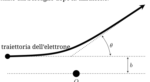Schema diffusione Rutherford con parametro b e angolo θ

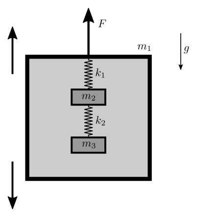Schema scatola nera con masse e molle

Topic: Electrostatics, Newtonian Mechanics Metodi: Coulomb’s Law, Experimental Data Analysis, Physical Modeling, Error Propagation, Graph Linearization Competenze: Experimental Data Analysis, Physical Reasoning Objects: Point Charge, Electron, Screen Fonte: Testo (PDF) — p.1 Soluzione: Soluzioni (PDF)

Problem 1 An unknown charge

1.1 Introduction

A point-form charge of unknown value $Q$ is held fixed in a region of space. Electrons are launched parallel to the $z$ axis from a distance from the charge and are diffused due to the electrostatic force produced by the fixed charge and then hit a detection screen. The details of the unknown charge can be known by varying the initial kinetic energy and initial coordinates $x_{i}$ and $y_{i}$ of the electron beam and measuring the final coordinates $x_{f}$ and $y_{f}$ of the point where the electron hits the finite-sized detection flat screen perpendicular to the $z$ axis and located at $z = 0$ .

It’s helpful to know the formula for the Rutherford distribution,

$b = \frac{k q Q}{2 E} \frac{1}{t a n ( θ /2 )}$

where $b$ is the impact parameter, $E$ is the electron energy, $q = - 1.602 \times 1 0^{- 19} C$ is the electron charge, $k = 8.99 \times 1 0^{9} N m^{2} / C^{2}$ , and $θ$ is the diffusion angle. The impact parameter is defined as the minimum distance of the electron from the target, assuming that the electron is not affected by the target and therefore moves in a straight line; the angle of diffusion is the angle between the initial velocity vector of the electron when it is far from the target and the final velocity vector of the electron far from the target after diffusion.

1.2 Purpose

The purpose is to determine the position $(x_{Q}, y_{Q}, z_{Q})$ and also the intensity and sign of the fixed charge $Q$ as accurately as possible. Approximate estimates and orders of magnitude of these results should be provided. There is a Gaussian error associated with the initial position of the beam of order $0.5 mm$ .

As with all experiments, you need to provide clearly labeled data tables, clearly labeled graphs, and derivations of enough formulas to explain what you’ve measured and how you’re getting the results.

1.3 Program interface

The program shall require that the acceleration voltage value be provided by the keyboard.

Beam accelerating voltage in V:

Enter a number between 1 and 10000 on the keyboard and press return. The programme then requires the initial starting coordinates, starting with $x_{i}$ :

x-coordinate of the electron beam in cm:

Enter a number between -20 and 20 on the keyboard and press return. Finally, the program requires the input of $y_{i}$ :

y-coordinate of the electron beam in cm:

Enter a number between -20 and 20 on the keyboard and press return. If an invalid number is entered in one of the three preceding cases, the program will reply Invalid entry. and ask for the value again, recalling the limits allowed.

After entering the three numbers, the program will provide:

Electron beam fired with parameters (x, y, V) =

and reaffirm the values entered, so:

Electron detected at (x, y) =

and it will indicate the position on the measured electron screen. However, if the electron does not hit the finite-sized screen, it will say:

Electron not detected...

The final programme is prepared to allow for the insertion of a new set of initial coordinates.

Rutherford diffusion scheme with parameter b and angle θ

Black box scheme with masses and springs

Problema 2 — Una scatola nera

2.1 Introduzione

Hai una scatola nera meccanica rigida composta da un recipiente di massa $m_{1}$ . All’interno del recipiente c’è un oggetto di massa $m_{2}$ appeso a una molla di massa trascurabile e di costante elastica $k_{1}$ che è fissata al soffitto della scatola. Un’altra massa $m_{3}$ è appesa alla massa $m_{2}$ tramite un’altra molla senza massa e di costante elastica $k_{2}$ . È presente una piccola resistenza viscosa che dipende dalla velocità degli oggetti. L’accelerazione di gravità della Terra è $g = 9.81 m/s^{2}$ ed è parallela ai lati della scatola.

La scatola può essere spostata verso l’alto o verso il basso con un’accelerazione costante a tratti. L’andamento dell’accelerazione può essere programmato tramite input fornendo la durata (in secondi) e l’accelerazione (in $m/s^{2}$ ) di ogni step. La simulazione mostra in “tempo reale” la forza $F$ esercitata sulla scatola necessaria per mantenere l’accelerazione data in quell’istante, insieme alla lettura del tempo. La simulazione registrerà anche le letture in un file di testo nella stessa cartella del programma. Tutte le simulazioni inizieranno sempre con la stessa configurazione iniziale per le masse.

Nota: Ogni misurazione della forza $F$ ha un piccolo errore casuale. Le molle sono lineari per deformazioni ragionevolmente piccole, ma non lineari per deformazioni maggiori. I valori $k_{1}$ e $k_{2}$ sono definiti come la costante elastica di ogni molla per piccole deformazioni vicine all’equilibrio quando la scatola è a riposo. La forza $F$ e l’accelerazione sono considerati positivi se diretti verso l’alto. La lunghezza del lato della scatola è $0.6 m$ e la scatola inizialmente si trova al centro di una stanza di altezza $3 m$ . Una simulazione termina automaticamente se la scatola colpisce il soffitto o il pavimento o se una delle masse si scontra con la scatola o con l’altra massa.

La figura non è disegnata in scala.

2.2 Scopo

Lo scopo è determinare tutti i parametri: $m_{1}$ , $m_{2}$ , $m_{3}$ , $k_{1}$ , $k_{2}$ . Non è necessario fornire un’analisi degli errori per questi risultati.

2.3 Interfaccia del programma

Inizialmente, il programma richiede una sequenza di input da tastiera. Hai le seguenti possibilità.

Inserire due numeri e premere return per aggiungere uno step all’andamento dell’accelerazione, per esempio: 1.5 -0.4. Il primo numero rappresenta la durata dello step in secondi (deve essere un multiplo di $0.01 s$ ) e il secondo numero rappresenta l’accelerazione in $m/s^{2}$ (deve essere compreso tra $- 30$ e $30$ ).
Inserire repeat e un numero intero e premere return per ripetere le azioni, per esempio: repeat 10. Il numero intero rappresenta il numero di volte che si vuole ripetere le azioni. Ogni azione ripetuta finisce con endrepeat.
Inserire endrepeat per terminare la ripetizione delle azioni.
Inserire sample e un numero e premere return per cambiare il tempo di campionamento, per esempio: sample 0.4. Il numero rappresenta il nuovo tempo di campionamento che è il tempo dopo il quale ogni nuova lettura è registrata in un file testo. Il tempo di campionamento deve essere un multiplo di $0.01 s$ , che è anche il tempo di campionamento di default.
Inserire begin per terminare la sequenza e iniziare la simulazione.

È anche possibile scrivere azioni multiple sulla stessa linea e quindi premere return. Per esempio, è possibile inserire:

sample 0.4 repeat 10 1.5 0.4 1.5 -0.4 endrepeat begin

per iniziare una simulazione dove si è cambiato il tempo di campionamento al valore $0.4 s$ e accelerare la scatola rispettivamente con $a = 0.4 m/s^{2}$ e $a = - 0.4 m/s^{2}$ 10 volte.

Se si inserisce un input non valido, si otterrà uno dei seguenti messaggi di errore:

Se l’accelerazione è fuori dall’intervallo permesso: Acceleration is out of range.
Se la durata dell’accelerazione è fuori dall’intervallo permesso: Duration is out of range.
Se il tempo di campionamento è fuori dall’intervallo permesso: Sampling time is out of range.
Se il numero di ripetizioni è fuori dall’intervallo permesso: Number of repeat times is out of range.
Se si prova a ripetere azioni all’interno di un’altra azione ripetuta: Cannot repeat actions inside another repeat.
Se si prova a terminare la ripetizione senza un’azione di fine ripetizione: Cannot end repeat outside repeat.
In tutti gli altri casi: Invalid entry.

Dopo aver inserito begin, il programma chiederà di inserire da tastiera un nome per il file di restituzione dei dati:

Enter name for output file (e.g. "results"). You should use Latin letters and numbers because some special characters are not allowed.

Inserire un nome e premere return. Le letture verranno salvate in un file .txt con il nome indicato nella stessa cartella del programma.

Successivamente, il programma visualizzerà Begin experiment. e inizia l’esperimento. Il programma visualizzerà quindi il tempo attuale dall’inizio dell’esperimento (Time (s)), il valore misurato della forza $F$ (Force (N)) e l’accelerazione della scatola (Accel (m/s^2)).

Il programma visualizzerà quindi uno dei seguenti messaggi:

Se la simulazione si è conclusa con successo: Experiment ended successfully.
Se la scatola tocca il soffitto: The box hit the ceiling. Experiment ended.
Se la scatola tocca il pavimento: The box hit the floor. Experiment ended.
Se le masse all’interno della scatola urtano tra loro o colpiscono le pareti della scatola: Masses and/or the box collided. Experiment ended.

Dopo la conclusione della simulazione è possibile iniziarne un’altra.

Topic: Oscillations & Waves, Newtonian Mechanics Metodi: Simple Harmonic Motion Analysis, Experimental Data Analysis, Physical Modeling, Free-Body Diagram, Hooke’s Law Competenze: Experimental Data Analysis, Physical Reasoning Objects: Container, Spring, Block Fonte: Testo (PDF) — p.1 Soluzione: Soluzioni (PDF)

Problem 2 A black box

2.1 Introduction to the book

Hai una scatola nera meccanica rigida composta da un recipiente di massa $m_{1}$ . Inside the container is an object of $m_{2}$ mass suspended from a spring of negligible mass and constant elasticity $k_{1}$ which is fixed to the ceiling of the box. Another mass $m_{3}$ is hung from the mass $m_{2}$ by another massless spring with an elastic constant $k_{2}$ . There is a small viscous resistance that depends on the speed of the objects. The Earth’s gravitational acceleration is $g = 9.81 m/s^{2}$ and is parallel to the sides of the box.

The box can be moved up or down with constant acceleration at stretches. The acceleration trend can be programmed by input providing the duration (in seconds) and acceleration (in $m/s^{2}$ ) of each step. The simulation shows in “real time” the force $F$ applied to the box necessary to maintain the acceleration given at that instant, together with the time reading. The simulation will also record readings in a text file in the same program folder. All simulations will always start with the same initial configuration for the masses.

Note: Each force measurement $F$ has a small random error. The springs are linear for reasonably small deformations but not linear for larger deformations. The values $k_{1}$ and $k_{2}$ are defined as the elastic constant of each spring for small deformations close to equilibrium when the box is at rest. The force $F$ and acceleration shall be considered positive if directed upwards. The length of the side of the box is $0.6 m$ and the box is initially located in the centre of a room of height $3 m$ . A simulation ends automatically if the box hits the ceiling or floor or if one of the masses collides with the box or the other mass.

The figure is not drawn in scale.

2.2 Purpose

The purpose is to determine all parameters: $m_{1}$ , $m_{2}$ , $m_{3}$ , $k_{1}$ , $k_{2}$ . It is not necessary to provide an error analysis for these results.

As with all experiments, you need to provide clearly labeled data tables, clearly labeled charts, and derivations of enough formulas to make clear what you’ve measured and how you’re getting the results.

2.3 Program interface

Initially, the program requires a sequence of keyboard inputs. You have the following options.

Enter two numbers and press return to add a step to the acceleration, for example: 1.5 -0.4. The first number represents the duration of the step in seconds (must be a multiple of $0.01 s$ ) and the second number represents the acceleration in $m/s^{2}$ (must be between $- 30$ and $30$ ).
Enter repeat and an integer and press return to repeat the actions, for example: repeat 10. The integer represents the number of times you want to repeat the actions. Each repeated action ends with endrepeat.
Insert endrepeat to finish the repetition of the actions.
Enter sample and a number and press return to change the sampling time, for example: sample 0.4. The number represents the new sampling time which is the time after which each new reading is recorded in a text file. The sampling time shall be a multiple of $0.01 s$ , which is also the default sampling time.
Enter begin to finish the sequence and start the simulation.

You can also write multiple actions on the same line and then press return. For example, you can insert:

sample 0.4 repeat 10 1.5 0.4 1.5 -0.4 endrepeat begin

to start a simulation where the sampling time has changed to $0.4 s$ and to accelerate the box by $a = 0.4 m/s^{2}$ and $a = - 0.4 m/s^{2}$ 10 times respectively.

If you enter an invalid input, you will get one of the following error messages:

If the acceleration is outside the range: `Acceleration is outside the range.
If the duration of acceleration is outside the allowed range: `Duration is out of range.
If the sampling time is outside the range: Sampling time is outside range.
If the number of repetitions is outside the allowed range: Number of repeat times is outside the allowed range.
If you try to repeat actions within another repeat action: Cannot repeat actions inside another repeat.
If you try to finish the repetition without an end repetition action: Cannot end repeat outside repeat.
In all other cases: `Invalid entry.

After entering begin, the program will ask to enter a name for the data return file from the keyboard:

Enter name for output file (e.g. "results"). You should use Latin letters and numbers because some special characters are not allowed.

Enter a name and press return. The readings will be saved in a file .txt with the name given in the same folder as the program.

The program will then display Begin experiment. and start the experiment. The program will then display the current time from the start of the experiment (Time (s) ), the measured value of the force $F$ (Force (N) ) and the acceleration of the box (Accel (m/s^2) ).

The program will then display one of the following messages:

If the simulation has been successfully completed: `Experiment ended successfully.
If the box hits the ceiling, the box hits the ceiling. Experiment ended. If the box hits the floor, the box hits the floor. Experiment ended.
If the masses inside the box collide with each other or hit the walls of the box: `Masses and/or the box collided. Experiment ended.

After the simulation is completed, another simulation can be started.

Raccolta Gare di Fisica

Esplora