EuPhO 2021 — Sperimentale

E1: Un filo nascosto

Apparato sperimentale e quesiti

Un filo di rame molto lungo corre orizzontalmente ad una profondità sconosciuta $h$ sotto una superficie quadrata orizzontale di lato pari a $L=100.0\text{mm}$. I lati del quadrato sono orientati Ovest-Est (asse $x$) e Sud-Nord (asse $y$), come mostrato in figura. L’origine del sistema di coordinate coincide con l’angolo sud-ovest del quadrato.

Il filo è collegato a una sorgente in corrente continua regolabile (non mostrata in figura), che può fornire una corrente $I$ nell’intervallo da $-5\text{A}$ a $5\text{A}$. L’inversione del segno della corrente corrisponde ad un’inversione della polarità della sorgente. Una piccola bussola può essere posizionata sulla superficie quadrata (che comprende la sua circonferenza) per rilevare il campo magnetico del filo attraverso l’angolo di deflessione $\phi$ tra l’ago magnetico e la direzione Nord ($y$). Valori $\phi$ positivi corrispondono ad una deflessione verso Est, come mostrato in figura, mentre $\phi$ negativi corrispondono ad una deflessione verso Ovest. Puoi supporre che:

• L’ago magnetico è un dipolo magnetico puntiforme, che può ruotare liberamente attorno all’asse verticale, cioè la bussola è sensibile solo alla componente orizzontale del campo magnetico.
• L’altezza dell’ago sopra la superficie è trascurabile rispetto alla profondità del filo sotto la superficie, cioè l’ago si trova nel piano $xy$.

Progetta il tuo esperimento ed effettua le simulazioni necessarie per eseguire le seguenti attività:

a. Determina l’orientamento del filo rispetto al sistema di coordinate specificandone l’equazione nella forma $y=ax+b$, e stima le incertezze dei parametri $a$ e $b$. Disegna la posizione del filo su un grafico e indica la direzione corrispondente alla corrente positiva $I$.

b. Determina la profondità $h$ del filo sotto la superficie e la componente orizzontale $B_E$ del campo magnetico terrestre. In questa attività non è necessario calcolare esplicitamente le incertezze sperimentali, tuttavia i risultati finali devono essere rappresentati con un numero appropriato di cifre significative.

La permeabilità magnetica del vuoto è ${\mu }_0=4\pi \times 10^{-7}\text{T m/A}$.

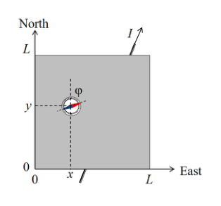Superficie quadrata con bussola e assi

Descrizione del software di simulazione

Il programma ”command line” simula la misurazione dell’angolo di deflessione $\phi$ dopo aver fornito la corrente $I$ e posizionato la bussola alle coordinate $x$ e $y$ sulla superficie.

Un tipico output di un singolo ciclo di simulazione del programma è il seguente:

Enter I (A) between -5.0 and 5.0: 3.4
Enter X (mm) between 0 and 100: 55
Enter Y (mm) between 0 and 100: 31
PHI = -33 degrees
-------------------------------
Enter I (A) between -5.0 and 5.0: _

Primo, inserisci la corrente $I$ in A (il numero tra $-5.0$ e $5.0$), poi le coordinate $x$ e $y$ in mm (i numeri tra 0 e 100). Ciascun input è confermato premendo il tasto Enter. Il programma fornirà in uscita il valore di $\phi$ (PHI) in gradi (arrotondato a $1^{\circ }$) e ritornerà allo stato iniziale.

La corrente inserita $I$ sarà arrotondata a $0.1\text{A}$, le coordinate inserite $x$, $y$ saranno arrotondate a $1\text{mm}$ prima di essere utilizzate nella simulazione. (Non vengono forniti punti nel tentativo di inserire numeri più precisi).

Ogni volta che cambi la posizione della bussola, la sua effettiva posizione usata nella simulazione differirà dalle coordinate inserite per un’incertezza di circa $0.5\text{mm}$. (È una simulazione della limitata precisione con cui si posiziona realmente un oggetto).

Ogni volta che hai necessità di uscire dal programma, premi Ctrl+C.

Topic: Magnetism Metodi: Physical Modeling, Experimental Data Analysis Competenze: Measurement & Instrumentation, Physical Reasoning Objects: Wire Fonte: Testo (PDF) — p.2 Soluzione: Soluzioni (PDF)

E1: Hidden wire

Experimental setup and tasks

A very long copper wire runs horizontally at unknown depth $h$ under a horizontal square surface of side length $L=100.0\text{mm}$. The sides of the square are oriented West-East (the $x$-axis) and South-North (the $y$-axis), as shown in the figure. The origin of the coordinate system coincides with the South-West corner of the square.

The wire is connected to an adjustable DC source (not shown in the figure), which can provide a current $I$ in the range from $-5\text{A}$ to $5\text{A}$. The reversal of the sign of the current corresponds to a reversal of the polarity of the source. A small compass can be placed on the square surface (including its circumference) to sense the magnetic field of the wire through the deflection angle $\phi$ between the magnetic needle and the North ($y$) direction. Positive $\phi$ values correspond to an Eastward deflection, as shown in the figure, while negative $\phi$ correspond to a Westward deflection. You can assume that:

• The magnetic needle is a point-like magnetic dipole, which can rotate freely around the vertical axis, i.e. the compass is sensitive to the horizontal component of the magnetic field only.
• The height of the needle above the surface is negligible compared to the depth of the wire beneath the surface, i.e. the needle is situated in the $xy$-plane.

Design your experiment and make the necessary simulations to perform the following tasks:

a. Determine the orientation of the wire with respect to the coordinate system by specifying its equation in the form $y=ax+b$, and estimate the uncertainties of the parameters $a$ and $b$. Draw the wire position on a graph and indicate the direction corresponding to a positive current $I$.

b. Determine the depth $h$ of the wire below the surface and the horizontal component $B_E$ of the Earth’s magnetic field. In this task you are not required to calculate the experimental uncertainties explicitly, however, your final results must be represented with an appropriate number of significant digits.

The magnetic permeability of free space is ${\mu }_0=4\pi \times 10^{-7}\text{T m/A}$.

Square surface with compass and axes

Description of the simulation software

The command line program simulates the measurement of the deflection angle $\phi$ after providing the current $I$ and placing the compass at the coordinates $x$ and $y$ on the surface.

A typical output of a single simulation cycle of the program looks like:

Enter I (A) between -5.0 and 5.0: 3.4
Enter X (mm) between 0 and 100: 55
Enter Y (mm) between 0 and 100: 31
PHI = -33 degrees
-------------------------------
Enter I (A) between -5.0 and 5.0: _

First, you enter the current $I$ in A (the number between $-5.0$ and $5.0$), then coordinates $x$ and $y$ in mm (the numbers between 0 and 100). Each input is confirmed with the Enter key. The program will output the value of $\phi$ (PHI) in degrees (rounded to $1^{\circ }$) and return to the initial prompt.

The current input $I$ will be rounded to $0.1\text{A}$, the coordinate inputs $x$, $y$ will be rounded to $1\text{mm}$ before being used in simulation. (There is no point in trying to input more precise numbers).

Every time you change the position of a compass, its real position used in simulation differs from the input coordinates with an error about $0.5\text{mm}$. (It is a simulation of a limited precision when you place an object).

Any time you need to quit the program, press Ctrl+C.

Topic: Magnetism Metodi: Physical Modeling, Experimental Data Analysis Competenze: Measurement & Instrumentation, Physical Reasoning Objects: Wire Fonte: Testo (PDF) — p.2 Soluzione: Soluzioni (PDF)

E2: Cilindro caldo

Introduzione

Un’asta metallica uniforme di lunghezza $L=30\text{cm}$ e raggio $r=1\text{cm}$ è costituita da un metallo sconosciuto e viene conservata a temperatura ambiente $T_0=26.9{}^{\circ }\text{C}=300\text{K}$. L’asta di metallo ha una massa $m=460\text{g}$. Il tuo compito è determinare le proprietà termiche del metallo sconosciuto. L’asta di metallo può essere riscaldata a una delle sue estremità e le misurazioni della temperatura possono essere eseguite in posizioni personalizzabili lungo l’asta. Il riscaldatore si trova tra $x=0$ e $x=L_h=3\text{cm}$ (vedi figura). Il riscaldatore può essere programmato specificando una potenza fissa (in watt) e la durata (in secondi) per la quale il riscaldatore viene acceso. Le misurazioni della temperatura vengono effettuate specificando fino a cinque posizioni per i sensori lungo l’asta, insieme alla frequenza, all’ora di inizio e all’ora di fine delle misurazioni. La simulazione mostrerà le letture della temperatura in ”tempo reale” accelerato (circa 10 volte più veloce rispetto al mondo reale).

Asta metallica con riscaldatore e sensori

Si può presumere che tutta la potenza di riscaldamento vada nell’asta e che l’asta perda calore nell’ambiente circostante tramite il trasferimento di calore con l’aria e la radiazione di corpo nero. Il trasferimento di calore con l’aria è lineare nella temperatura dell’asta e può essere descritto da un coefficiente $\alpha$ tale che il trasferimento di calore per unità di area e per unità di tempo è $\alpha (T-T_0)$. L’aria è ben ventilata in modo che si possa assumere che $\alpha$ sia costante su tutta la superficie dell’asta e indipendente dalla temperatura della superficie. La perdita di calore tramite radiazione di corpo nero può essere descritta usando la legge di Stefan-Boltzmann modificata con emissività $\beta$ tale che la perdita di calore per radiazione per unità di area e per unità di tempo è $\beta \sigma (T^4-T_0^4)$, dove $\sigma =5.67\times 10^{-8}{\text{W/(m}}^2{\text{K}}^4)$. Similmente ad $\alpha$, si può assumere che l’emissività sia costante in tutta l’asta e indipendente dalla temperatura. L’asta è inoltre caratterizzata dalla conducibilità termica $k$ (tale che il flusso di calore lungo $x$ è $-kdT/dx$) e dal calore specifico $c$.

Quesito

Il compito è determinare il calore specifico del metallo sconosciuto, $c$ (unità $\text{J/(K kg)}$), la conduttività termica $k$ (unità $\text{W/(m K)}$), e i coefficienti della perdita di calore $\alpha$ (unità ${\text{W/(m}}^2\text{K)}$) e $\beta$ (adimensionale). Dovresti tentare di trovare i valori in un intervallo di incertezza del 10 % del valore vero. Questo perché ci sono varie fonti di errore, come le fluttuazioni gaussiane sia nella definizione delle posizioni dei sensori, sia nelle misurazioni della temperatura. Le dimensioni degli errori possono essere trovate osservando le fluttuazioni nell’output.

Come per tutti gli esperimenti, devi fornire tabelle di dati chiaramente etichettate, grafici chiaramente etichettati e derivazioni di formule sufficienti per chiarire cosa hai misurato e come stai ricavando i tuoi risultati.

Topic: Thermodynamics Metodi: First Law of Thermodynamics, Physical Modeling Competenze: Mathematical Modeling, Experimental Data Analysis Objects: — Fonte: Testo (PDF) — p.2 Soluzione: Soluzioni (PDF)

E2: Hot Cylinder

Introduction

A uniform metal rod of length $L=30\text{cm}$ and radius $r=1\text{cm}$ is made of an unknown metal and is kept at room temperature $T_0=26.9{}^{\circ }\text{C}=300\text{K}$. The metal rod is weighed to be $m=460\text{g}$. Your task is to determine the thermal properties of the unknown metal. The metal rod can be heated at one of its ends, and temperature measurements can be performed on customizable locations along the rod. The heater is located between $x=0$ and $x=L_h=3\text{cm}$ (see fig). The heater can be programmed by specifying a fixed power (in watts) and the duration (in seconds) for which the heater is turned on for. Temperature measurements are made by specifying up to five locations for the sensors along the rod, alongside with the frequency, starting time and the ending time of the measurements. The simulation will show the temperature readings in accelerated ”real time” (running around 10 times faster than in the real world).

Metal rod with heater and sensors

You may assume that all of the heating power goes into the rod, and that the rod loses heat to its surroundings via heat transfer with air and black body radiation. Heat transfer with air is linear in temperature of the rod, and can be described by a coefficient $\alpha$ such that the heat transfer per unit area per unit time is $\alpha (T-T_0)$. The air is well-ventilated such that $\alpha$ can be assumed to be constant throughout the surface of the rod and independent of the temperature of the surface. Heat loss via black body radiation can be described using the Stefan-Boltzmann law modified with emissivity $\beta$ such that the heat loss to radiation per unit area per unit time is $\beta \sigma (T^4-T_0^4)$, where $\sigma =5.67\times 10^{-8}{\text{W/(m}}^2{\text{K}}^4)$. Similar to $\alpha$, the emissivity can be assumed to be constant throughout the rod, and independent of temperature. The rod is further characterised by the thermal conductivity $k$ (such that the heat flux density along $x$ is $-kdT/dx$) and the specific heat capacity $c$.

Task

The task is to determine the specific heat of the unknown metal, $c$ (units $\text{J/(K kg)}$), the thermal conductivity $k$ (units $\text{W/(m K)}$), and the heat loss coefficients $\alpha$ (units ${\text{W/(m}}^2\text{K)}$) and $\beta$ (dimensionless). You should aim to find the values within 10 % of the true value. This is because there are various sources of errors, such as Gaussian fluctuations in both defining the locations of the sensors, and the taking the temperature measurements. The sizes of the errors can be found by observing the fluctuations in the output.

As with all experiments, you must provide clearly labelled tables of data, clearly labelled graphs, and sufficient formulae derivations to make it clear what you have measured, and how you are deriving your results.

Topic: Thermodynamics Metodi: First Law of Thermodynamics, Physical Modeling Competenze: Mathematical Modeling, Experimental Data Analysis Objects: — Fonte: Testo (PDF) — p.2 Soluzione: Soluzioni (PDF)

Interfaccia del programma

L’esecuzione del programma di simulazione, denominato rod, consente di eseguire più esperimenti sull’asta. Il programma chiederà una sequenza di richieste di inserimento dati riguardanti l’impostazione dell’esperimento. Per ogni prompt, devono essere immessi i valori corrispondenti, quindi premere return per passare al prompt successivo. I prompt sono i seguenti:

1. La potenza di riscaldamento del riscaldatore: Enter P (W), between 0 and 300:
2. La durata dopo l’inizio dell’esperimento per la quale il riscaldatore è acceso (dopo questo tempo, il riscaldatore sarà spento): Enter heating duration (s), between 0 and 3600s:
3. I tempi di inizio e fine (dopo l’inizio dell’esperimento) per le misurazioni della temperatura effettuate sull’asta: Enter the starting and finishing time for the measurements (s), separated by a space. Must be between 0 e 3600s:

Topic: Thermodynamics Metodi: First Law of Thermodynamics, Physical Modeling Competenze: Mathematical Modeling, Experimental Data Analysis Objects: Rod Fonte: Testo (PDF) — p.2 Soluzione: Soluzioni (PDF)

Program interface

Running the simulation program, named rod, allows performing multiple experiments on the rod. The program will ask a sequence of prompts regarding the setup of the experiment. For each prompt, the corresponding value(s) should be entered, followed by pressing return to go the next prompt. The prompts are as follows:

1. The heating power of the heater:

Enter P (W), between 0 and 300:

2. The duration after the start of the experiment for which the heater is turned on for (after this time, the heater will be turned off):

Enter heating duration (s), between 0 and 3600s:

3. The starting and finishing times (after the start of the experiment) for the temperature measurements made on the rod:

Enter the starting and finishing time for the measurements (s), separated by a space. Must be between 0 and 3600s:

Topic: Thermodynamics Metodi: First Law of Thermodynamics, Physical Modeling Competenze: Mathematical Modeling, Experimental Data Analysis Objects: Rod Fonte: Testo (PDF) — p.2 Soluzione: Soluzioni (PDF)

4. L’intervallo di tempo tra due misurazioni consecutive effettuate con i sensori di temperatura: Enter dt (s), between 5 and 3600s and a multiple of 5s:

Topic: Thermodynamics Metodi: Physical Modeling, Experimental Data Analysis Competenze: Mathematical Modeling, Measurement & Instrumentation Objects: — Fonte: Testo (PDF) — p.2 Soluzione: Soluzioni (PDF)

4. The time interval between two consecutive measurements that are made with the temperature sensors:

Enter dt (s), between 5 and 3600s and a multiple of 5s:

Topic: Thermodynamics Metodi: Physical Modeling, Experimental Data Analysis Competenze: Mathematical Modeling, Measurement & Instrumentation Objects: — Fonte: Testo (PDF) — p.2 Soluzione: Soluzioni (PDF)

5. Le posizioni dei sensori di temperatura lungo l’asta. Le coordinate sono specificate rispetto alla fine del riscaldatore: Enter up to 5 locations for the sensors (in cm), between L=0 and L=30cm, separated by spaces: Nota che non inserire alcun numero significa semplicemente non effettuare alcuna misurazione.

Topic: Thermodynamics Metodi: Physical Modeling, Experimental Data Analysis Competenze: Mathematical Modeling, Measurement & Instrumentation Objects: Rod Fonte: Testo (PDF) — p.2 Soluzione: Soluzioni (PDF)

5. The locations of the temperature sensors along the rod. The coordinates are specified with respect to the end with the heater:

Enter up to 5 locations for the sensors (in cm), between L=0 and L=30cm, separated by spaces:

Note that not entering any numbers simply means not taking any measurements.

Topic: Thermodynamics Metodi: Physical Modeling, Experimental Data Analysis Competenze: Mathematical Modeling, Measurement & Instrumentation Objects: Rod Fonte: Testo (PDF) — p.2 Soluzione: Soluzioni (PDF)

6. Il nome del file di output per le letture della temperatura. Nota che tutte le letture salvate verranno visualizzate anche sullo schermo: Enter the output file name: Si consiglia di utilizzare solo lettere e numeri latini per il nome. Altri caratteri possono o non possono essere consentiti nel nome del file e in caso di un nome di file non valido, le letture non verranno salvate. Le letture verranno salvate in un file .txt con il nome dato nella stessa cartella del programma. Se si inserisce un input non valido, verrà inviato un messaggio di errore chiarificatore e verrà data un’altra opportunità di inserimento. Il programma chiederà quindi di premere return per avviare l’esperimento, o digitare restart e premere return per reinserire tutti i parametri sperimentali. Dopo aver continuato con la simulazione, il programma visualizzerà un riepilogo della configurazione sperimentale, quindi inizierà a mostrare il tempo trascorso dall’accensione del riscaldatore (t(s)) e tutte le letture del sensore nello stesso ordine in cui sono stati inseriti nel prompt ($T_i$(°C), dove $i$ corrisponde all’$i$-esimo sensore). Al termine della simulazione, è possibile avviare un nuovo esperimento digitando restart e premendo return.

Topic: Thermodynamics Metodi: Physical Modeling, Experimental Data Analysis Competenze: Measurement & Instrumentation, Experimental Data Analysis Objects: — Fonte: Testo (PDF) — p.2 Soluzione: Soluzioni (PDF)

6. The output file name for the temperature readings. Note that all of the saved readings will also be displayed on the screen:

Enter the output file name:

You are advised to only use Latin letters and numbers for the name. Other characters may or may not be allowed in the filename and in case of an invalid filename, the readings will not be saved. The readings will be saved in a .txt file with the given name in the same folder as the program.

If you enter an invalid input, a clarifying error message will be sent, and an another opportunity for entering the input will be given.

The program will then prompt to press return to start the experiment, or typing restart and pressing return to re-enter all the experimental parameters. After continuing with the simulation, the program will display a summary of the experimental setup, and then start printing out the time elapsed since the heater was turned on (t(s)), and all the sensor readings in the same order they were entered in the prompt ($T_i$(°C), where $i$ corresponds to the $i$-th sensor).

After the simulation ends, a new experiment can be started by typing restart and pressing return.

Topic: Thermodynamics Metodi: Physical Modeling, Experimental Data Analysis Competenze: Measurement & Instrumentation, Experimental Data Analysis Objects: — Fonte: Testo (PDF) — p.2 Soluzione: Soluzioni (PDF)