OII na Teorica

Theory Q1-1 Italiano (Italy) Caratterizzazione dei colloidi del suolo (10 punti) La scienza dei colloidi è utile per caratterizzare le particelle del suolo poiché molte di loro possono essere trattate come particelle colloidali di dimensione micrometrica. Ad esempio, il moto browniano (moto casuale delle particelle colloidali) può essere utilizzato per misurare le dimensioni delle particelle. Parte A. Moto delle particelle colloidali (1.6 punti) Analizziamo il moto browniano unidimensionale di una particella colloidale di massa M. L’equazione del moto per la sua velocità v(t) è: Ṁv= $-\gamma v(t$) + F(t) + Fext(t), (1) dove γè il coefficiente di attrito, F(t) è una forza dovuta alle collisioni casuali con le molecole d’acqua ed Fext(t) è una forza esterna. Nella Parte A, assumeremo Fext(t) = 0. A.1 Si consideri che una molecola d’acqua urti la particella a t= t0, dando un impulso I0, e dopo di ciò F(t) = 0. Se prima dell’urto v(t) = 0, per t> t0 v(t) = $v0e-(t-t0)/\tau$. Determinare v0 e τ, utilizzando I0e i parametri presenti nell’Eq (1). 0.8pt Nel seguito si potrà utilizzare τnelle risposte. A.2 In realtà, le molecole d’acqua si scontrano con la particella una dopo l’altra. Supponiamo che la i-sima collisione dia impulso Iial tempo tie determinare v(t) a condizione che t> 0 e v(0) = 0. Si fornisca inoltre la disuguaglianza che specifica l’intervallo di tiche deve essere considerato per un dato t. Nel foglio risposte non è necessario specificare questo intervallo nell’espressione per v(t). 0.8pt Parte B. Equazione efficace del moto (1.8 punti) I risultati ottenuti finora implicano che le velocità delle particelle v(t) e $v(t^{\prime }$) possono essere considerate quantità casuali e non correlate se $|t-t^{\prime }|\gg \tau$. Su questa base introduciamo un modello teorico per descrivere approssimativamente il moto browniano unidimensionale dove la velocità cambia casualmente e ad ogni intervallo di tempo $\delta (\gg \tau$), ossia, v(t) = vn $(tn-1$ < $t\text{leqtn}$), (2) con tn= nδ(n= 0, 1, 2, ⋯) e vnè un una quantità casuale. Quest’ultimo soddisfa $\text{langlevn}⟩=$ 0, $\text{langlevnvm}⟩=$ {C (n= m), 0 $(n\text{neqm}$), (3) dove Cè un parametro dipendente da δ. Qui la scrittura $\text{langleX}\text{rangleindica}$ il valor medio di X. Ciò vuol dire che se estraiamo dei numeri casuali Xinfinite volte, il loro valor medio sarà $\text{langleX}⟩$. Si consideri ora lo spostamento della particella $\text{Deltax}(t$) = $x(t)-x(0$) per t= Nδdove Nè un numero intero. B.1 Si determini $⟨\text{Deltax}(t)\text{ranglee}⟨\text{Deltax}(t)2\text{ranglein}$ funzione di C, δ, e t. 1.0pt

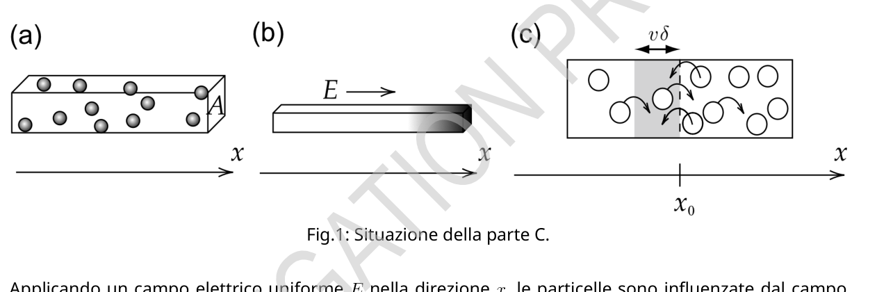
Theory Q1-2 Italiano (Italy) B.2 La quantità $⟨\text{Deltax}(t)2\text{rangleviene}$ chiamato spostamento quadratico medio (Mean Square Displacement MSD). È una quantità caratteristica osservabile del moto browniano, che corrisponde al caso limite in cui $\delta \to 0$. Da questo si può mostrare che $C\propto \delta \alpha e⟨\text{Deltax}(t)2⟩\text{proptot}\beta$. Si determinino i valori di αe β. 0.8pt Parte C. Elettroforesi (2.7 punti) Qui si discute l’elettroforesi cioè il trasporto di particelle cariche a causa di un campo elettrico. Una sospensione di particelle colloidali con massa Me carica Q(> 0) viene posta in uno stretto canale avente una sezione trasversale A(Fig. 1(a)). Ignoriamo l’interazione tra le particelle, gli effetti delle pareti, gli ioni presenti lì e la gravità. Fig.1: Situazione della parte C. Applicando un campo elettrico uniforme Enella direzione x, le particelle sono influenzate dal campo elettrico e la loro concentrazione n(x) (numero di particelle per unità di volume) diventa non-uniforme (Fig.1(b)). Se Eviene rimosso, questa non-uniformità scompare gradualmente. Questo è dovuto al moto browniano delle particelle. Se n(x) non è uniforme, il numero di particelle che si muovono verso destra può essere diverso da quello delle particelle che si muovono verso sinistra (Fig.1(c)). Questo origina un flusso di particelle JD(x), definito come il numero medio di particelle per unità di area trasversale e per unità di tempo nel punto xche si muovono lungo l’asse x. Questo flusso soddisfa la relazione JD(x) = $-Ddn$ dx(x), (4) dove Dviene chiamato coefficiente di diffusione. Si assuma ora per semplicità che metà delle particelle abbiano velocità +ve l’altra metà abbia velocità $-v$. Sia N+(x0) il numero di particelle con velocità +vper unità di superficie trasversa e per unità di tempo che attraversano x0 da sinistra a destra. Affinché le particelle con velocità +vattraversino x0 nell’intervallo di tempo δesse devono essere contenute nella regione grigia di Fig.1(c). Poiché δè piccolo, si ottiene n(x) $\text{simeqn}(x0$) + $(x-x0$) dn dx(x0) in questa regione. C.1 Si determini N+(x0) utilizzando le opportune quantità tra le seguenti v, δ, n(x0), e dn dx(x0). 0.5pt Definiamo $N-(x0$) come la controparte di N+(x0) per la velocità $-v$. Con ciò, abbiamo JD(x0) = $\text{langleN}+(x0)-$ $N-(x0)⟩$. In base all’Eq.(3), abbiamo $\text{langlev}2⟩=$ C.

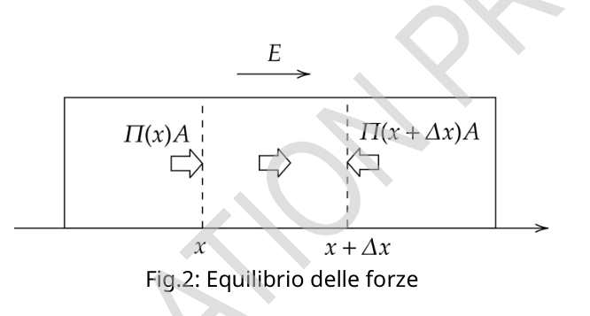
Theory Q1-3 Italiano (Italy) C.2 Determinare JD(x0) utilizzando le quantità necessarie tra le seguenti C, δ, n(x0) e dn dx(x0). Utilizzando questa relazione e la Eq.(4), si esprima Dcome funzione di Ce δ, $e⟨\text{Deltax}(t)2\text{ranglecome}$ funzione di De t. 0.7pt Discutiamo ora l’effetto della pressione osmotica $\Pi$. Risulta data da $\Pi$ = n NART= nkTin termini della costante di Avogadro NA, la costante universale dei gas R, la temperatura T, e la costante di Boltzmann k= R NA. Si consideri la concentrazione non uniforme causata dal campo elettrico E(Fig.1(b)). Poiché n(x) dipende da x, lo stesso vale per $\Pi (x$). Allora le forze causate da $\Pi (x$) e $\Pi (x+\text{Deltax}$) devono essere equilibrate dalla forza totale causata dal campo Eche agisce sulle particelle (Fig.2). Qui si suppone $\text{Deltax}$ piccolo, cosicché n(x) può essere considerato costante in questo intervallo, mentre n(x+ $\text{Deltax}$) $-n(x$) $\simeq$ $\text{Deltaxdn}$ dx(x). Fig.2: Equilibrio delle forze C.3 Si esprima dn dx(x) utilizzando n(x), T, Q, E, e k. 0.5pt Si discuta ora il bilancio del flusso. Oltre al flusso JD(x) causato dal moto browniano, è presente un flusso causato dal campo elettrico JQ(x). Esso è dato da JQ(x) = n(x)u, (5) dove uè la velocità terminale delle particelle sotto l’influsso del campo. C.4 Per determinare u, si utilizza la Eq.(1) con Fext(t) = QE. Poiché v(t) fluttua, consideriamo $\text{langlev}(t)⟩$. Assumendo $\text{langlev}(0)⟩=$ 0 e utilizzando $\text{langleF}(t)⟩=$ 0, si calcoli $\text{langlev}(t)\text{ranglee}$ si ottenga u= $limt\to \infty \text{langlev}(t)⟩$. 0.5pt C.5 L’equazione di bilancio del flusso implica JD(x) + JQ(x) = 0. Si esprima il coefficiente di diffusione Din funzione di k, γ, e T. 0.5pt Parte D. Spostamento quadratico medio (2.4 punti) Si supponga di osservare il moto browniano di una particella colloidale isolata, sferica, con raggio a= 5.0 μm in acqua. La figura 3 mostra gli istogrammi degli spostamenti $\text{Deltaxmisurati}$ nella direzione xa intervalli regolari $\text{Deltat}=$ 60 s . Il coefficiente di attrito è dato da γ= 6πaηcon viscosità dell’acqua η= 8.9 $\times 10-4$ Pa $\cdots$ e temperatura T= 25 ∘C.

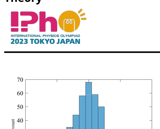
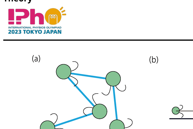
Theory Q1-4 Italiano (Italy) Fig.3: Istogramma degli spostamenti. D.1 Dai dati della Fig.3, stimare il valore di NAf ino a due cifre significative senza utilizzare il fatto che si tratta della costante di Avogadro. La costante dei gas è R= 8.31 J/K $\text{cdotmol}$. Non utilizzare il valore della costante di Boltzmann kdata nelle Istruzioni Generali. Per quanto riguarda la costante di Avogadro si potrebbe ottenere un valore differente da quello nelle Istruzioni Generali. 1.0pt Ora si estende il modello della parte B per descrivere il moto di una particella dotata di carica Qsotto l’azione di un campo elettrico E. La velocità della particella v(t) considerata nella Eq.(2) dovrebbe essere sostituita da v(t) = u+ $vn(tn-1$ < $t\text{leqtn}$) dove vnsoddisfa la Eq. (3) e uè la velocità limite considerata nella Eq.(5). D.2 Esprimere la MSD (spostamento quadratico medio) $⟨\text{Deltax}(t)2\text{ranglein}$ termini di u, D e te ricavane il comportamento asintotico per piccoli valori di te grandi valori di t, nonché il tempo caratteristico t∗in cui si verifica questo cambiamento. Tracciare un grafico approssimativo della MSD in un grafico log-log, indicando la posizione approssimativa di t∗. 0.8pt Si considerino poi i microbi che nuotano (Fig. 4(a)), per semplicità in una sola dimensione (Fig. 4(b)). Si tratta di particelle sferiche di raggio a. In ogni intervallo di tempo δ, ogni microbo

p.2 — Situazione della parte L, elettroforesi

p.3 — Forze agenti sulla particella colloidale

p.4 — Istogramma degli spostamenti

p.5 — Movimento del microbo (a) e (b)

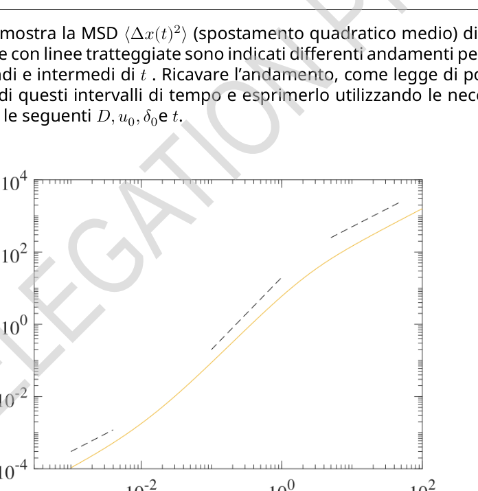
p.5 — Spostamento quadratico medio dei microbi

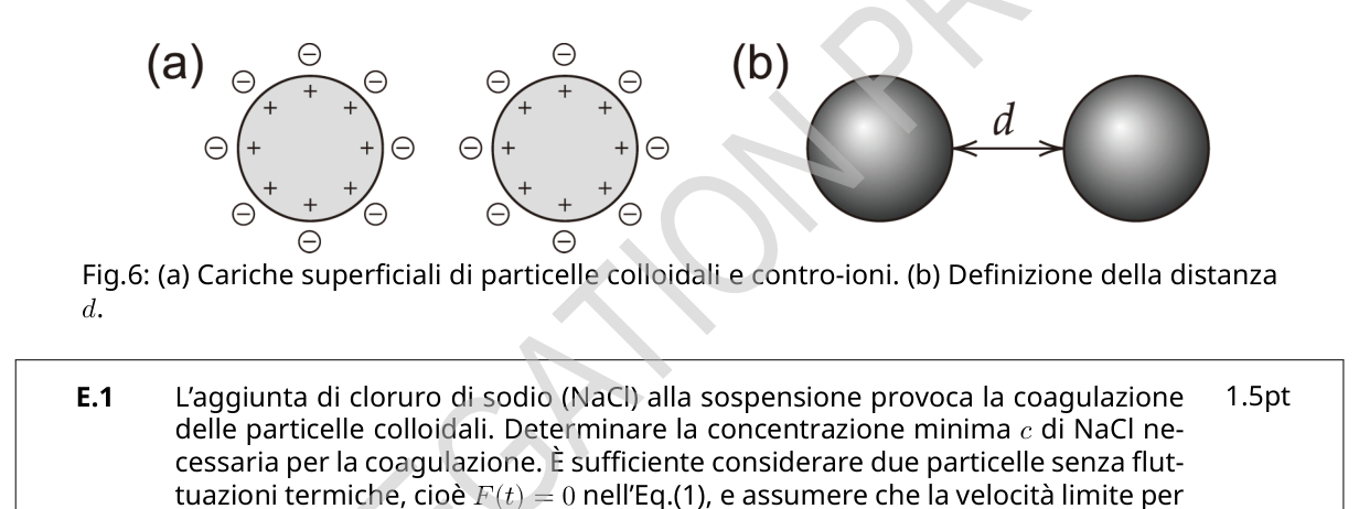
p.6 — Cariche superficiali e definizione distanza d

Topic: Kinetic Theory, Thermodynamics, Electrostatics Metodi: Differential Equations, Impulse-Momentum Theorem, Statistical Averaging, Experimental Data Analysis Competenze: Mathematical Modeling, Physical Reasoning, Experimental Data Analysis Objects: — Fonte: Testo (PDF) — p.1 Soluzione: Soluzioni (PDF)

Theory Q1-1 Italian (Italy) Characterisation of soil colloids (10 points) Colloid science is useful for characterizing soil particles because many of them can be treated as colloidal particles of micrometric size. For example, the Brownian motion (motor) The coloidal particle size of the sample is calculated by measuring the particle size of the sample. Part A. The motion of colloidal particles (1.6 points) We’re going to analyze the one-dimensional Brownian motion of a colloidal particle of mass M. The equation of the motor for its speed v(t) is: Ṁv= $-\gamma v(t$) + F(t) + Fext(t), (1) where γ is the friction coefficient, F(t) is a force due to accidental collisions with water molecules and Fext(t) is an external force. In Part A, we’re going to assume Fext(t) = 0. A.1 Consider that a water molecule hits the particle at t=t0, giving a Pulse I0, and then F(t) = 0. If before the impact v(t) = 0, per t> t0 v(t) = $v0e-(t-t0)/\tau$. Determine v0 and τ using the parameters in the Eq (1). 0.8pt The following answers can be used. A.2 In fact, water molecules collide with the particle one after the other. Suppose the i-th collision gives momentum and time to determine v condition that t> 0 and v(0) = 0. The inequality specifying the range of tics to be considered for a given t is also provided. In the reply sheet This interval need not be specified in the expression for v(t). 0.8pt Part B. Effective equation of the motorcycle (1.8 points) The results so far imply that the particle velocities v(t) and $v(t^{\prime }$) can be considered as Random and unrelated quantities if $|t-t^{\prime }|\gg \tau$. On this basis, we introduce a theoretical model to describe approximately one-dimensional Brownian motion where velocity changes randomly. and at each time interval $\delta (\gg \tau$), i.e. v(t) = vn $(tn-1$ < $t\text{leqtn}$), (2) with tn=nδ(n=0, 1, 2, ) and there’s a random quantity. The latter satisfies $\text{langlevn}⟩=$ 0, $\text{langlevnvm}⟩=$ {C (n= m), 0 $(n\text{neqm}$), (3) where there is a dependent parameter of δ. Here, write $\text{langleX}\text{rangleindica}$ the mean of X. This means that If we take random numbers Xinfinite times, their mean value is $\text{langleX}⟩$. Now consider the displacement of the particle $\text{Deltax}(t$) = $x(t)-x(0$) by t= Nδwhere N is an integer. B.1 Determine the $⟨\text{Deltax}(t)\text{ranglee}⟨\text{Deltax}(t)2\text{ranglein}$ function of C, δ, and t. 1.0pt

Theory Q1-2 Italian (Italy) B.2 The amount $⟨\text{Deltax}(t)2\text{rangleviene}$ called average squared displacement (Mean) Square Displacement MSD). It is an observable characteristic quantity of brownian motion, corresponding to the limit case where $\delta \to 0$. This is the way to go. to show that $C\propto \delta \alpha e⟨\text{Deltax}(t)2⟩\text{proptot}\beta$. The values of αe β are determined. 0.8pt Part C. The following table shows the results of the calculation: The problem is that the electric field is the transport of charged particles. A colloidal particle suspension with mass Me charge Q(> 0) is placed in a narrow channel having a cross section A(Fig. 1(a)). We ignore the interaction between particles, the effects of walls, ions. It’s there and gravity. Figure 1: Situation of Part C. Applying a uniform electric field in the direction x, the particles are affected by the field Electrical and their concentration n(x) (number of particles per unit volume) becomes non-uniform (Fig. 1 (b)) If Eviene is removed, this non-uniformity will gradually disappear. This is because of the bike. Brownish particles. If n(x) is not uniform, the number of particles moving to the right The resulting particle size is the same as the particle size of the particle size of the particle size of the particle size of the particle size of the particle size of the particle size of the particle size of the particle size of the particle size of the particle size of the particle size of the particle size of the particle size of the particle size of the particle size of the particle size of the particle size of the particle size of the particle size of the particle size of the particle size of the particle size of the particle size of the particle size of the particle size of the particle size of the particle size of the particle size of the particle size of the particle size of the particle size of the particle size of the particle size of the particle size of the particle size of the particle size of the particle size of the particle size of the particle size of the particle size of the particle size of the particle size of the particle size of the particle size of the particle size of the particle size of the particle size of the particle size of the particle size of the particle size of the particle size of the particle size of the particle size of the particle size of the particle size of the particle size of the particle size of the particle size of the particle size of the particle size of the particle size of the particle size of the particle size of the particle size of the particle size of the particle size of the particle size of the particle size of the particle size of the particle size of the particle size of the particle size of the particle of the particle of the particle size of the particle of the particle of the left. This gives rise to a Particle flow JD(x), defined as the average number of particles per unit area crossed and for units of time at the point x that move along the x-axis. This flow satisfies the report JD(x) = $-Ddn$ dx(x), (4) where it’s called the spread coefficient. It is now assumed for simplicity that half of the particles have velocities + and the other half has velocities $-v$. Either N+(x0) the number of particles with velocity +v per unit of cross-sectional area and per unit of time which They’re going through x0 from left to right. So that the particles with speed + pass through x0 in the range The time δ must be contained in the grey region of Fig.1(c). Since δ is small, you get n(x) $\text{simeqn}(x0$) + $(x-x0$) dn dx(x0) in this region. C.1 N+(x0) shall be determined using the appropriate quantities between the following v, δ, n(x0), e dn dx(x0). 0.5pt We define $N-(x0$) as the counterpart of N+(x0) for the speed $-v$. With that, we have JD(x0) = $\text{langleN}+(x0)-$ $N-(x0)⟩$. According to Eq.(3), we have $\text{langlev}2⟩=$ C.

Theory Q1-3 Italian (Italy) C.2 Determine JD(x0) using the necessary quantities between the following C, δ, n(x0) e dn dx(x0). Using this relation and Eq. Ce δ, $e⟨\text{Deltax}(t)2\text{ranglecome}$ funzione di De t. 0.7pt Let us now discuss the effect of osmotic pressure $\Pi$. The result is given by $\Pi$ = n The following terms are used: Avogadro’s constant NA, the universal gas constant R, the temperature T, and the Boltzmann constant k= R NA. Consider the non-uniform concentration caused by the electric field E(Fig.1(b)). Because n(x) depends on x, the same is true for $\Pi (x$). Then the forces caused by $\Pi (x$) and $\Pi (x+\text{Deltax}$) must be The resulting force is the total force of the Eche field acting on the particles (Fig. 2). This is assumed to be $\text{Deltax}$ So small, so that n(x) can be considered constant in this range, while n(x+ $\text{Deltax}$) $-n(x$) $\simeq$ $\text{Deltaxdn}$ dx(x). Fig. 2: Balance of forces C.3 It is expressed as dx(x) using n(x), T, Q, E, and k. 0.5pt The current budget is being discussed. In addition to the JD(x) flow caused by the Brownian motion, a flow is present caused by the electric field JQ(x). It is given by JQ(x) = n(x)u, (5) where the particle’s terminal velocity under the influence of the field is. C.4 To determine u, we use the equation Eq.(1) with Fext(t) = QE. Since v(t) fluctuates, we consider $\text{langlev}(t)⟩$. Assuming $\text{langlev}(0)⟩=$ 0 and using $\text{langleF}(t)⟩=$ 0, $\text{langlev}(t)\text{ranglee}$ is calculated The resulting value is u= $limt\to \infty \text{langlev}(t)⟩$. 0.5pt C.5 The flow balance equation implies JD(x) + JQ(x) = 0. The following is the Diffusion coefficient Din function of k, γ, and T. 0.5pt The following is the list of the following: Average square displacement (2.4 points) Suppose we observe the Brownian motion of an isolated, spherical colloidal particle with a radius of a= 5.0 μm in water. Figure 3 shows histograms of the $\text{Deltaxmisurati}$ movements in the xa direction intervalli regolari $\text{Deltat}=$ 60 s . The friction coefficient is given by γ= 6πaηcon viscosity of the water η= 8.9 $\times 10-4$ Pa $\cdots$ e temperatura T= 25 ∘C.

Theory Q1-4 Italian (Italy) Figure 3: Istogram of the movements. D.1 From Fig.3, estimate the value of NAf in two significant digits without So we’re going to use the fact that this is Avogadro’s constant. The gas constant is R= 8.31 J/K $\text{cdotmol}$. Do not use the value of the Boltzmann constant given in the General Instructions. As for Avogadro’s constant, you could The Commission shall, in particular, examine the results of the studies and the results of the studies. 1.0pt Now we extend the model of Part B to describe the motion of a charged particle Qsotto The action of an electric field E. The velocity of the particle v(t) taken into account in Eq. replaced by v(t) = u+ $vn(tn-1$ < $t\text{leqtn}$) where the Eq is satisfied. (3) and u is the speed limit considered in Eq.(5). D.2 Express the MSD (mean square displacement) $⟨\text{Deltax}(t)2\text{ranglein}$ terms of u, D And you got the asynthetic behavior for small values of your big values The time of the change shall be the time of the change. Draw an approximate MSD graph in a log-log graph, indicating the approximate position of t. 0.8pt The following are the microbes that swim. 4 (a)), for simplicity in one dimension (Fig. 4(b)). Si It is spherical particles of radius a. In each time interval δ, each microbes

p.2 — Situazione della parte L, elettroforesi

p.3 — Forze agenti sulla particella colloidale

p.4 — Istogramma degli spostamenti

p.5 — Movimento del microbo (a) e (b)

p.5 — Spostamento quadratico medio dei microbi

p.6 — Cariche superficiali e definizione distanza d

Topic: Kinetic Theory, Thermodynamics, Electrostatics Metodi: Differential Equations, Impulse-Momentum Theorem, Statistical Averaging, Experimental Data Analysis Competenze: Mathematical Modeling, Physical Reasoning, Experimental Data Analysis Objects: — Fonte: Testo (PDF) — p.1 Soluzione: Soluzioni (PDF)