Problem T1. Zero gravity (10 points)

In all your subsequent calculations, you may use the following physical constants and their numerical values.

The radius of Earth $R_{\oplus} = 6.4 \times 1 0^{6} m$ .
Free fall acceleration at the sea level $g = 9.81 m/s^{2}$ .

Part A. Zero-g flight (3 points)

Astronauts can experience weightlessness during their space-flight. However, there is a cheaper way to experience weightlessness other than boarding a spaceship: there are airplanes specifically designed to create weigthlessness on board during a certain time period. Such an airplane is shown in the photo.

For this Part, the following values can be also used.

The speed of sound at the flying altitude $c_{s} = 300 m/s$ .
The altitude (from the sea level) at which the airplane starts zero-g-flight (the flight segment during which the objects on board the aircraft have zero weight) is $h_{0} = 7600 m$ .
The speed of the airplane when it starts zero-g-flight is $v_{0} = 460 km/h$ .
The angle between the horizontal plane and the direction of the velocity vector at the moment when the airplane starts zero-g-flight $α_{0} = 4 7^{\circ}$ .

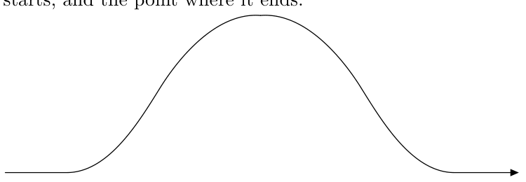
i. (0.5 pts) Below is a sketch of a zero-g flight trajectory (the one providing the longest duration of weightlessness might be slightly different). Mark on it the point where zero-g flight starts, and the point where it ends.

ii. (0.5 pts) What should be the direction and magnitude of the acceleration of the airplane to ensure that the passengeres would feel weightlessness?

iii. (0.5 pts) What is the speed of the airplane at the highest point of its trajectory?

iv. (0.5 pts) How long does it take for the airplane to reach the highest point on its trajectory from the moment when it starts zero-g-flight?

v. (0.5 pts) What is the altitude of the airplane at the highest point of its trajectory from the sea level?

vi. (0.5 pts) The possible values of the initial speed $v_{0}$ and initial ascending angle $α_{0}$ are limited by the robustness of the airplane’s construction, and by the maximal thrust provided by the engines; the numerical values given above can be considered to be optimal, i.e. yielding the longest period during which the passengers experience weightlessness. Assuming that there are no restrictions on the final diving angle (the angle between the horizontal plane and the direction of the velocity vector at the moment when the airplane ends zero-g-flight) while the only limitation on the speed is that it cannot be larger than the speed of sound, what is the maximal total duration of a zero-g flight segment?

Part B. Glass of water in weightlessness (3 points)

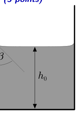
Consider a partially filled glass of water on board this aircraft. The glass is cylindrical, of radius $r = 3 cm$ ; the walls of the glass are negligibly thin. At the moment when the airplane starts zero-g flight, the water surface is flat except for the small meniscus of negligible height near the walls of the glass (see the figure depicting axial cross-section of the glass), and the depth of water is $h_{0} = 3 cm$ . The contact angle of the water in the glass (the angle between the tangent to the water surface and the surface of the glass at the point where the water surface and glass are in direct contact, see the figure) is $β = 0^{\circ}$ (the figure is illustrative).

i. (1 pt) Under the condition of weightlessness, the water surface will take a new equilibrium shape. Sketch the shape of the water surface at the axial cross-section of the glass.

ii. (1 pt) What is the minimal distance between the water surface and the bottom of the glass at the new equilibrium state?

iii. (1 pt) Under normal conditions, this glass can hold up to $V_{0} = 200 ml$ water. What is the maximal volume of water which can be held in this glass in weightlessness? Sketch also the corresponding shape of the water surface at the axial cross-section of the glass.

Part C. Sharpshooter on geostationary orbit (4 points)

Weightlessness can be experienced also on spaceships performing ballistic motion (motion when engines are switched off). Let us consider an astronaut on geostationary orbit. This is a circular orbit around Earth which lies in the equatorial plane, and the period of motion on which is equal to $T_{0} = 24 h$ .

i. (0.7 pts) What is the radius of the geostationary orbit?

ii. (1.8 pts) For research reasons, the astronaut wants to hit his own spaceship with a bullet fired from a rifle equipped onto the spaceship. The speed of the bullet leaving the rifle is $u_{0} = 1200 m/s$ , the bullet’s velocity lies on the orbital plane. Under which angle with respect to the vector pointing towards the centre of the Earth does he needs to aim the rifle if he wants to hit the spaceship within the next 40 hours? You don’t need to prove that there is only one suitable shooting angle.

You may use the expression for the total energy of an elliptical orbit, $E_{total} = - \frac{G M _{\oplus} m}{2 a}$ , where $a$ is the semi-major axis.

iii. (1.5 pts) He also tries out another rifle the bullet speed of which can be freely adjusted from zero to the maximal speed $u_{m} = 300 m/s$ . With this rifle, he aims strictly along the motion of the spaceship. What is the bullet’s smallest possible travel time until hitting the spaceship?

Fonte: Testo (PDF) — p.1

Topic: Gravitation, Newtonian Mechanics Metodi: Kepler’s Laws, Newton’s Law of Gravitation, Kinematic Equations, Conservation of Energy Competenze: Physical Reasoning, Mathematical Modeling, Diagrammatic Reasoning Objects: Container, Satellite, Projectile

Problem T1. Zero gravity (10 points)

In tutti i tuoi successivi calcoli, puoi usare le seguenti costanti fisiche e i loro valori numerici.

The radius of Earth $R_{\oplus} = 6.4 \times 1 0^{6} m$ .
Free fall acceleration at the sea level $g = 9.81 m/s^{2}$ .

Parte A. Zero-g flight (3 punti)

Gli astronauti possono sperimentare l’assenza di peso durante il loro volo spaziale. Tuttavia, c’è un modo più economico per sperimentare l’assenza di peso diverso da imbarcarsi in una nave spaziale: ci sono aerei specificamente progettati per creare assenza di peso a bordo durante un certo periodo di tempo. Such an airplane è mostrato nella foto.

Per questa parte, si possono utilizzare anche i seguenti valori.

La velocità del suono a quota di volo $c_{s} = 300 m/s$ .
L’altitudine (dal livello del mare) a cui l’aereo inizia il volo zero-g (il segmento di volo durante il quale gli oggetti a bordo dell’aereo hanno peso zero) è $h_{0} = 7600 m$ .
La velocità dell’aereo quando inizia il volo zero-g è $v_{0} = 460 km/h$ .
The angle between the horizontal plane and the direction of the velocity vector at the moment when the airplane starts zero-g-flight $α_{0} = 4 7^{\circ}$ .

**i. (0.5 pts) ** Below is a sketch of a zero-g flight trajectory (the one providing the longest duration of weightlessness might be slightly different). Marcare il punto in cui inizia il volo zero-G, e il punto in cui finisce.

ii. (0.5 pts) What should be the direction and magnitude of the acceleration of the airplane to ensure that the passengeres would feel weightlessness?

iii. (0.5 pts) What is the speed of the airplane at the highest point of its trajectory?

iv. (0.5 pts) How long does it take for the airplane to reach the highest point on its trajectory from the moment when it starts zero-g-flight?

v. (0.5 pts) What is the altitude of the airplane at the highest point of its trajectory from the sea level?

**vi. (0.5 pts) ** I possibili valori della velocità iniziale $v_{0}$ e dell’angolo ascendente iniziale $α_{0}$ sono limitati dalla robustezza della costruzione dell’aeroplano e dalla massima spinta fornita dai motori; i valori numerici di cui sopra possono essere considerati ottimali, cioè rendendo il periodo più lungo durante il quale i passeggeri sperimentano l’assenza di peso. Supponendo che non ci siano restrizioni sull’angolo di immersione finale (l’angolo tra il piano orizzontale e la direzione del vettore di velocità al momento in cui l’aereo termina il volo zero-g), mentre l’unica limitazione sulla velocità è che non può essere maggiore della velocità del suono, qual è la durata totale massima di un segmento di volo zero-g?

Parte B. Glass of water in weightlessness (3 punti)

Considerate un bicchiere partialmente riempito di acqua a bordo di questo aereo. Il vetro è cilindrico, di raggio $r = 3 cm$ ; le pareti del vetro sono trascurabilmente sottili. Al momento in cui l’aereo inizia il volo zero-g, la superficie dell’acqua è piana, tranne che per il piccolo menisco di altezza negligible vicino alle pareti del vetro (vedi la figura che raffigura la sezione trasversale asiale del vetro), e la profondità dell’acqua è $h_{0} = 3 cm$ . L’angolo di contatto dell’acqua nel vetro (l’angolo tra la tangente alla superficie dell’acqua e la superficie del vetro al punto in cui la superficie dell’acqua e il vetro sono in contatto diretto, vedere la figura) è $β = 0^{\circ}$ (la figura è illustrativa).

**i. (1 pt) ** In condizione di weightlessness, la superficie dell’acqua assumirà una nuova forma di equilibrio. Sketta la forma della superficie dell’acqua alla sezione trasversale asseiale del vetro.

ii. (1 pt) What is the minimal distance between the water surface and the bottom of the glass at the new equilibrium state?

**iii. (1 pt) ** In condizioni normali, questo vetro può contenere $V_{0} = 200 ml$ acqua. Qual è il volume massimo di acqua che può essere tenuto in questo bicchiere in assenza di peso? Sketta anche la forma corrispondente della superficie dell’acqua alla sezione trasversale asiale del vetro.

Parte C. Sharpshooter in orbita geostationaria (4 punti)

La mancanza di peso può essere sperimentata anche su navi spaziali che eseguono movimento balistico (mozione quando i motori sono spenti). Consideriamo un astronauta in orbita geostazionaria. Questa è un’orbita circolare intorno alla Terra che si trova nel piano equatoriale, e il periodo di movimento su cui è uguale a $T_{0} = 24 h$ .

i. (0.7 pts) What is the radius of the geostationary orbit?

ii. (1.8 pts) For research reasons, the astronaut wants to hit his own spaceship with a bullet fired from a rifle equipped onto the spaceship. La velocità del proiettile che lascia il fucile è $u_{0} = 1200 m/s$ , la velocità del proiettile è sul piano orbitale. In quale angolo rispetto al vettore che punta verso il centro della Terra deve puntare il fucile se vuole colpire la nave spaziale entro le prossime 40 ore? Non c’è bisogno di dimostrare che c’è un solo angolo di tiro adatto.

Si può usare l’espressione per l’energia totale di un’orbita ellittica, $E_{total} = - \frac{G M _{\oplus} m}{2 a}$ , dove $a$ è l’asse semi-maggiore.

**iii. (1.5 pts) ** Egli prova anche un’altra rifle the bullet speed of which can be freely adjusted from zero to the maximum speed $u_{m} = 300 m/s$ . Con questo fucile, mira rigorosamente lungo il movimento della nave spaziale. Qual è il tempo di viaggio più piccolo possibile fino a quando non colpirà la nave spaziale?

Fonte: Testo (PDF) — p.1

Problem T1. Zero gravity (10 points)

In all your subsequent calculations, you may use the following physical constants and their numerical values.

The radius of Earth $R_{\oplus} = 6.4 \times 1 0^{6} m$ .
Free fall acceleration at sea level $g = 9.81 m/s^{2}$ .

Part A. Zero-g flight (3 points)

Astronauts can experience weightlessness during their spaceflight. However, there is a cheaper way to experience weightlessness other than boarding a spaceship: there are airplanes specifically designed to create weightlessness on board during a certain time period. Such an airplane is shown in the photo.

For this part, the following values can also be used.

The speed of sound at the flying altitude $c_{s} = 300 m/s$ .
The altitude (from sea level) at which the aircraft starts zero-g flight (the flight segment during which the objects on board the aircraft have zero weight) is $h_{0} = 7600 m$ .
The speed of the aircraft when it starts zero-g flight is $v_{0} = 460 km/h$ .
The angle between the horizontal plane and the direction of the velocity vector at the moment when the aircraft starts zero-g flight $α_{0} = 4 7^{\circ}$ .

ii. (0.5 pts) What should be the direction and magnitude of the acceleration of the airplane to ensure that the passengeres would feel weightlessness?

iii. (0.5 pts) What is the speed of the airplane at the highest point of its trajectory?

**iv. (0.5 pts) ** How long does it take for the aircraft to reach the highest point on its trajectory from the moment it starts zero-g flight?

v. (0.5 pts) What is the altitude of the airplane at the highest point of its trajectory from the sea level?

vi. (0.5 pts) The possible values of the initial speed $v_{0}$ and initial ascending angle $α_{0}$ are limited by the robustness of the airplane’s construction, and by the maximal thrust provided by the engines; the numerical values given above can be considered to be optimal, i.e. yielding the longest period during which the passengers experience weightlessness. Assuming that there are no restrictions on the final diving angle (the angle between the horizontal plane and the direction of the velocity vector at the moment when the plane ends zero-g flight) while the only limitation on the speed is that it cannot be greater than the speed of sound, what is the maximum total duration of a zero-g flight segment?

Part B. Glass of water in weightlessness (3 points)

Consider a partially filled glass of water on board this aircraft. The glass is cylindrical, of radius $r = 3 cm$ ; the walls of the glass are negligibly thin. At the moment when the aircraft starts zero-g flight, the water surface is flat except for the small meniscus of negligible height near the walls of the glass (see the figure depicting axial cross-section of the glass), and the depth of water is $h_{0} = 3 cm$ . The angle of contact of the water in the glass (the angle between the tangent to the water surface and the surface of the glass at the point where the water surface and glass are in direct contact, see the figure) is $β = 0^{\circ}$ (the figure is illustrative).

i. (1 pt) Under the condition of weightlessness, the water surface will take a new equilibrium shape. Sketch the shape of the water surface at the axial cross-section of the glass.

ii. (1 pt) What is the minimal distance between the water surface and the bottom of the glass at the new equilibrium state?

iii. (1 pt) Under normal conditions, this glass can hold up to $V_{0} = 200 ml$ water. What is the maximum volume of water that can be held in this glass in weightlessness? Sketch also the corresponding shape of the water surface at the axial cross-section of the glass.

Part C. Sharpshooter on geostationary orbit (4 points)

Weightlessness can also be experienced on spacecraft performing ballistic motion (motion when engines are switched off). Let’s consider an astronaut on geostationary orbit. This is a circular orbit around Earth which lies in the equatorial plane, and the period of motion on which is equal to $T_{0} = 24 h$ .

**i. (0.7 pts) ** What is the radius of the geostationary orbit?

ii. (1.8 pts) For research reasons, the astronaut wants to hit his own spaceship with a bullet fired from a rifle equipped onto the spaceship. The speed of the bullet leaving the rifle is $u_{0} = 1200 m/s$ , the bullet’s velocity lies on the orbital plane. Under what angle with respect to the vector pointing towards the center of the Earth does he need to aim the rifle if he wants to hit the spaceship within the next 40 hours? You don’t need to prove that there’s only one suitable shooting angle.

You may use the expression for the total energy of an elliptical orbit, $E_{total} = - \frac{G M _{\oplus} m}{2 a}$ , where $a$ is the semi-major axis.

iii. (1.5 pts) He also tries out another rifle the bullet speed of which can be freely adjusted from zero to the maximal speed $u_{m} = 300 m/s$ . With this rifle, he’s aiming strictly along the motion of the spaceship. What is the bullet’s smallest possible travel time until hitting the spaceship?

Fonte: Testo (PDF) — p.1

Problem T2. Controlled fusion (11 points)

In all your subsequent calculations, you may use the following physical constants and their numerical values.

Boltzmann constant $k_{B} = 1.381 \times 1 0^{- 23} J \cdot K^{- 1}$
Elementary charge $e = 1.602 \times 1 0^{- 19} C$
Electron’s mass $m_{e} = 9.109 \times 1 0^{- 31} kg$
Planck’s constant $h = 6.626 \times 1 0^{- 34} m^{2} \cdot kg \cdot s^{- 1}$
Permittivity of free space $ϵ_{0} = 8.854 \times 1 0^{- 12} F \cdot m^{- 1}$

Nuclear fusion is a reaction where light atomic nuclei merge to form a larger nucleus. The difference in the rest energies of the fusing nuclei and the fusion product is released as heat. For instance, if deuterium (consisting of one neutron and one proton, denoted as D) and tritium (consisting of two neutrons and one proton, denoted as T) merge, they will form an $α$ -particle, a neutron, and 14 MeV of energy. While humans have learned how to ignite fusion reaction explosively in hydrogen bombs, they are still struggling to succeed in controlled fusion, i.e. to control fusion reaction so that the released heat could be used for operating power plants. The most feasible reaction for a controlled fusion is the above mentioned D-T reaction which will be addressed by this Problem.

Part A. General considerations (0.5 points)

In what follows, we shall express the temperature in electron volts; this is a common practice for so high temperatures. 1 eV corresponds to such a temperature $T$ by which the characteristic thermal energy $k_{B} T$ equals to the potential energy of an electron in electrostatic potential of $V = 1 V$ .

For a power plant, the released fusion energy must be larger than the total energy loss. It can be shown that for an optimally designed D-T reactor (device in which the controlled fusion takes place), the temperature of the deuterium and tritium nuclei should be $T_{0} = 14 keV$ while the product of the number density of particles $n$ (the number of particles per volume) and the confinement time $τ$ (the time during which density $n$ remains roughly constant) should not be less than $2 \times 1 0^{20} s/m^{3}$ ; this requirement is know as the Lawson criterion. The main techonlogical challenge is to achieve a long enough confinement of the hot plasma.

i. (0.5 pts) Express the fusion temperature $T_{0}$ in Kelvins.

Part B. Tokamak (2.5 points)

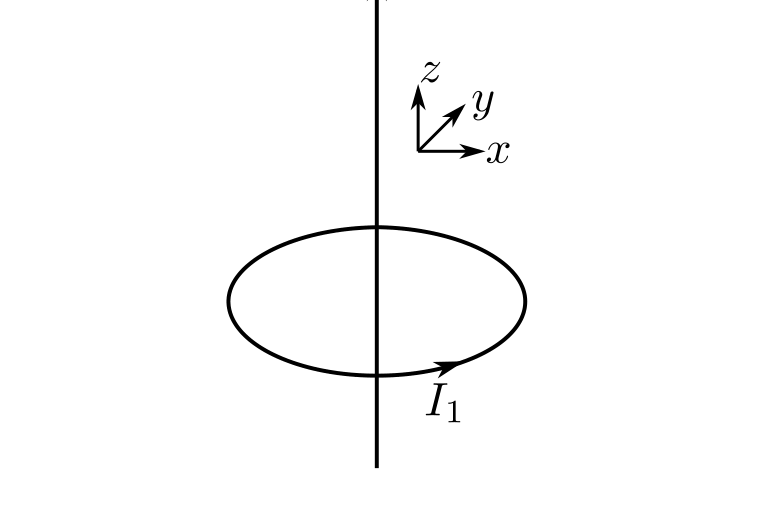
The most popular design of fusion reactors is tokamak. In a tokamak, charged particles move along magnetic field lines and are confined because the field lines are confined into a finite volume of space. Qualitatively, the magnetic field lines have the same shape as in the case of an infinitely long straight current passing coaxially through a circular current loop. In the following subtasks, you’re expected to provide the sketches in a 3d projection as shown in the figure.

i. (0.5 pts) Sketch magnetic field lines of a infinitely long straight current.

ii. (0.5 pts) Sketch magnetic field lines of a circular current loop.

iii. (0.75 pts) Sketch a magnetic field line of an infinitely long straight current passing coaxially through a circular current loop which starts from a small distance from the circular current.

iv. (0.75 pts) For the same current configuration as before, sketch a magnetic field line starting from a small distance from the straight current.

Part C. Cold fusion (3.5 points)

“Cold fusion” refers to a muon-catalytic fusion process by which an electron in a hydrogen molecule (which can include one deuterium and one tritium nucleus) is substituted by a muon. Muon, having a 207 times larger mass than an electron, brings the nuclei in the molecule closer to each other, thereby increasing the probability of their fusion. The idea of such a catalytic fusion was suggested in 1947-48 by A. Sakharov and F.C. Frank, and lead to a short-lived research boom in 1989 after an erraneous report of a successful fusion at room temperatures by M. Fleischmann and S. Pons. The problem with muon-catalytic fusion is that the energetic cost of producing one muon is larger than the total energy released by fusion reaction mediated by one muon; the possible solutions are either decreasing the energetic cost of a muon, or increasing the number of fusions mediated by a single muon. In what follows, we consider a simple approach to understand why substituting electrons with muons will decrease the size of an atom.

i. (1 pt) Using classical mechanics and considering an electron on a circular orbit of radius $R$ around a point-like nucleus of charge $+ 2 e$ , relate the momentum $p$ of the electron to the orbit’s radius $R$ .

ii. (1 pt) At the ground state, the total energy is as small as possible; meanwhile, the state of the electron (muon) cannot violate the uncertainty principle. From these considerations, find an estimate for the radius $R$ at the ground state.

iii. (1 pt) By the subtask i, we neglected the distance between the two nuclei in the molecule which was permissable for estimating the orbital radius $R$ . Now, however, we want also to get an estimate for the distance between the nuclei. To that end, consider another simple model. The two electrons (muons) on their orbit form a ball-like cloud: let us assume that there is a spherical ball of radius $R$ carrying a total charge $- 2 e$ , homogeneously distributed over the entire volume of the ball. Inside the charged ball, there are two nuclei which can be considered as point masses and point charges (of charge $+ e$ each), able to move frictionlessly inside the ball. Find the equilibrium distance $d$ between the nuclei.

iv. (0.5 pts) Based on the model suggested above, by how many times is the distance between the deuterium and tritium atoms reduced when orbital electrons are substituted by muons?

Part D. Inertial confinement fusion (4.5 points)

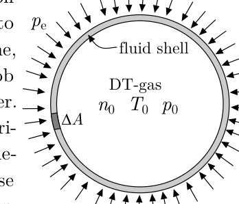
Third approach to controlled fusion is based on the idea that due to mass and inertia, it takes some time, although short, for any hot blob of matter to explode and scatter. In order to satisfy the Lawson criterion one can inrease the confinement time, but one can also increase the number density $n$ . In the inertial confinement fusion devices, powerful beams are used to create highly compressed balls of gas of densities exceeding the density of lead by hundreds of times. In what follows, we consider this approach by adopting a simple model: a liquid spherical shell of total mass $M$ and radius $r$ is surrounding a ball of gas of number density $n_{0}$ , temperature $T_{0}$ , and pressure $p_{0} = k_{B} n_{0} T_{0}$ (in reality, the shell is solid, but at really high pressures, solids essentially liquify); see the figure. Each gas molecule consists of a deuterium nucleus, tritium nucleus, and two electrons. The thickness of the walls of the spherical liquid shell $δ$ is much smaller than $r$ ( $δ ≪ r$ ).

i. (0.5 pts) Consider a small piece of shell of surface area $Δ A$ . Express its mass in terms of the quantities introduced above.

ii. (1 pt) External pressure $p_{e}$ ( $p_{e} ≫ p_{0}$ ) is applied to the shell. Express the initial acceleration of a small piece of the shell in terms of the quantities introduced until now.

iii. (1.5 pts) While the shell contracts due to external pressure, the pressure inside grows, and at a certain moment, it becomes larger than the external pressure. Express the minimal radius of the shell $r_{m}$ and the maximal temperature inside the shell $T_{m}$ (which are achieved when the surrounding shell stops for a moment before reversing its direction of motion) in terms of the quantities introduced above. Keep in mind that the inside temperature becomes so high that the gas is converted into a completely ionized plasma made of nuclei and electrons. You may assume that $p_{e}$ remains constant during the entire process (this might not be entirely true, but under this assumption, we shall still be able to get a correct order of magnitude for the answer), the shell contracts while retaining its spherical shape, and the thermal energy transferred to the shell can be neglected.

iv. (1.5 pts) The huge external pressure $p_{e}$ is created by irradiating the shell from outside, isotropically from all sides, with a laser of total output power $P$ . As a result, the outer layers of the shell are evaporated, and the evaporated atomic nulcei flow away at the average speed of $u$ . Estimate the pressure $p_{e}$ in terms of $P$ , $r$ , and $u$ ; you may assume that $u$ is much smaller than the speed of light.

Fonte: Testo (PDF) — p.1

Topic: Nuclear & Particle Physics, Modern-Quantum Physics Metodi: Bohr Model & Quantization, Coulomb’s Law, Free-Body Diagram, Order-of-Magnitude Estimation Competenze: Physical Reasoning, Mathematical Modeling, Estimation & Approximation, Diagrammatic Reasoning Objects: Nucleus, Electron, Gas

Problem T2. Controlled fusion (11 points)

In tutti i tuoi successivi calcoli, puoi usare le seguenti costanti fisiche e i loro valori numerici.

Boltzmann costante $k_{B} = 1.381 \times 1 0^{- 23} J \cdot K^{- 1}$
Elementary charge $e = 1.602 \times 1 0^{- 19} C$
massa di elettrone $m_{e} = 9.109 \times 1 0^{- 31} kg$
Planck’s constant $h = 6.626 \times 1 0^{- 34} m^{2} \cdot kg \cdot s^{- 1}$
Permittivity of free space $ϵ_{0} = 8.854 \times 1 0^{- 12} F \cdot m^{- 1}$

La fusione nucleare è una reazione in cui i nuclei di luce si uniscono per formare un nucleo più grande. La differenza tra le energie rimanenti dei nuclei di fusione e il prodotto di fusione viene rilasciata come calore. Per esempio, se deuterium (consistente di un neutrone e un protone, denotato come D) e tritium (consistente di due neutroni e un protone, denotato come T) si uniscono, formano una particella $α$ , un neutrone, e 14 MeV di energia. Mentre gli umani hanno imparato a accendere la reazione di fusione esplosivamente nelle bombe ad idrogeno, stanno ancora lottando per riuscire nella fusione controllata, cioè per controllare la reazione di fusione in modo che il calore rilasciato possa essere utilizzato per le centrali elettriche in funzione. La reazione più fattibile per una fusione controllata è la reazione D-T sopra menzionata che sarà affrontata da questo problema.

Parte A. Considerazioni generali (0,5 punti)

In ciò che segue, esprimeremo la temperatura in elettroni volts; questa è una pratica comune per temperature così elevate. 1 eV corrisponde a una temperatura $T$ in cui la caratteristica energia termica $k_{B} T$ è uguale all’energia potenziale di un elettrone in potenziale elettrostatico di $V = 1 V$ .

Per un impianto di energia, l’energia di fusione rilasciata deve essere maggiore del totale di perdita di energia. Si può dimostrare che per un reattore D-T (dispositivo in cui si svolge la fusione controllata) ottimamente progettato, la temperatura dei nuclei di deuterio e tritio dovrebbe essere $T_{0} = 14 keV$ mentre il prodotto del numero di densità di particelle $n$ (il numero di particelle per volume) e il tempo di confinamento $τ$ (il tempo durante il quale la densità $n$ rimane approssimativamente costante) non dovrebbe essere inferiore a $2 \times 1 0^{20} s/m^{3}$ ; questo requisito è noto come criterio di Lawson. La sfida tecnologico principale è quella di raggiungere un confinamento abbastanza lungo del plasma caldo.

**i. (0,5 pts) ** Express the fusion temperature $T_{0}$ in Kelvins.

Parte B. Tokamak (2.5 punti)

Il progetto più popolare dei reattori di fusione è Tokamak. In un tokamak, le particelle cariche si muovono lungo linee di campo magnetico e sono confinate perché le linee di campo sono confinate in un volume finito di spazio. Qualitativamente, le linee del campo magnetico hanno la stessa forma di una corrente continua infinitamente lunga che passa coaxialmente attraverso un loop di corrente circolare. Nei seguenti sotto-tasche, si prevede di fornire gli schizzi in una proiezione 3D come mostrato nella figura.

i. (0.5 pts) Sketch magnetic field lines of a infinitely long straight current.

**ii. (0.5 pts) ** Sketch magnetic field lines of a circular current loop.

**iii. (0.75 pts) ** Sketta una linea di campo magnetico di una corrente diretta infinitamente lunga passando coaxialmente attraverso un loop di corrente circolare che inizia da una piccola distanza dalla corrente circolare.

**iv. (0.75 pts) ** Per la stessa configurazione corrente come prima, disegnare una linea di campo magnetico partendo da una piccola distanza dal corrente dritta.

Parte C. Fusione a freddo (3,5 punti)

“Fusione fredda” si riferisce a un processo di fusione catalitica di muoni in cui un elettrone in una molecola di idrogeno (che può includere un deuterium e un nucleo di tritium) è sostituito da un muone. Il muone, avendo una massa 207 volte maggiore di un elettrone, porta i nuclei della molecola più vicini l’uno all’altro, aumentando così la probabilità della loro fusione. L’idea di una fusione catalytica simile fu suggerita nel 1947-48 da A. Sakharov e F.C. Frank, and lead to a short-lived research boom nel 1989 after an erroneous report of a successful fusion at room temperatures by M. Carnivore e S. Pons. Il problema con la fusione catalitica di muoni è che il costo energetico di produrre un muone è maggiore del totale di energia rilasciata dalla reazione di fusione mediata da un muone; le possibili soluzioni sono diminuire il costo energetico di un muone o aumentare il numero di fusioni mediate da un singolo muone. In questo, consideriamo un approccio semplice per capire perché sostituire gli elettroni con muoni diminuirà la dimensione di un atomo.

**i. (1 pt) ** Usando la meccanica classica e considerando un elettrone su un’orbita circolare di radius $R$ intorno a un nucleo di carica point-like $+ 2 e$ , relate il momento $p$ dell’elettrone al radius $R$ dell’orbita.

**ii. (1 pt) ** allo stato di base, l’energia totale è il più piccolo possibile; nel frattempo, lo stato dell’elettrone (muon) non può violare il principio di incertezza. Da queste considerazioni, trovare un estimate per il raggio $R$ allo stato di base.

**iii. (1 pt) ** Per il subtask i, abbiamo trascurato la distanza tra i due nuclei nella molecola che era permissabile per la stima del raggio orbitale $R$ . Ora, tuttavia, vogliamo anche ottenere una stima per la distanza tra i nuclei. Per questo, consideriamo un altro modello semplice. The two electrons (muons) on their orbit form a ball-like cloud: let us assume that there is a spherical ball of radius $R$ carrying a total charge $- 2 e$ , homogeneously distributed over the entire volume of the ball. All’interno della palla carica, ci sono due nuclei che possono essere considerati come masse puntate e cariche puntate (di carica $+ e$ ciascuno), capaci di muoversi senza attrito all’interno della palla. Trova la distanza di equilibrio $d$ tra i nuclei.

iv. (0.5 pts) Based on the model suggested above, by how many times is the distance between the deuterium and tritium atoms reduced when orbital electrons are substituted by muons?

Parte D. Fusione a confinamento inertio (4.5 punti)

Terzo approccio alla fusione controllata si basa sull’idea che a causa della massa e dell’inerzia, ci vuole un po’ di tempo, sebbene breve, per qualsiasi blocco di materia caldo esplodere e disperdere. Per soddisfare il criterio di Lawson si può aumentare il tempo di confinamento, ma si può anche aumentare la densità di numero $n$ . Nei dispositivi di fusione a confinamento inerziale, i potenti raggi sono utilizzati per creare palline di gas altamente compresse di densità che superano la densità del piombo di centinaia di volte. In ciò che segue, consideriamo questo approccio adottando un modello semplice: una conchiglia sferica liquida di massa totale $M$ e raggio $r$ circonda una sfera di gas di densità numerosa $n_{0}$ , temperatura $T_{0}$ , e pressione $p_{0} = k_{B} n_{0} T_{0}$ (in realtà, la conchiglia è solida, ma a pressioni davvero elevate, solidi essenzialmente liquidi); vedi la figura. Ogni molecola di gas è composta da un nucleo di deuterio, un nucleo di tritio e due elettroni. The thickness of the walls of the spherical liquid shell $δ$ is much smaller than $r$ ( $δ ≪ r$ ).

i. (0.5 pts) Consider a small piece of shell of surface area $Δ A$ . Esprimere la sua massa in termini di quantità introdotte sopra.

**ii. (1 pt) ** Pressione esterna $p_{e}$ ( $p_{e} ≫ p_{0}$ ) è applicata alla conchiglia. Esprimere l’accelerazione iniziale di un piccolo pezzo del guscio in termini di quantità introdotte fino ad ora.

iii. (1.5 pts) While the shell contracts due to external pressure, the pressure inside grows, and at a certain moment, it becomes larger than the external pressure. Esprimere il minimo raggio della conchiglia $r_{m}$ e la temperatura massima all’interno della conchiglia $T_{m}$ (che sono raggiunti quando la conchiglia circostante si ferma per un momento prima di invertere la sua direzione di movimento) in termini dei quantitativi introdotti sopra. Tenete presente che la temperatura interna diventa così alta che il gas viene convertito in un plasma completamente ionizzato fatto di nuclei ed elettroni. Si può supporre che $p_{e}$ rimanga costante durante l’intero processo (questo potrebbe non essere completamente vero, ma sotto questa ipotesi, saremo ancora in grado di ottenere un ordine corretto di magnitudo per la risposta), la conchiglia si contrae mantenendo la sua forma sferica, e l’energia termica trasferita alla conchiglia può essere trascurata.

iv. (1.5 pts) The huge external pressure $p_{e}$ is created by irradiating the shell from outside, isotropically from all sides, with a laser of total output power $P$ . Di conseguenza, gli strati esterni della conchiglia vengono evaporati e i nulcei atomici evaporati scorrono alla velocità media di $u$ . Estimare la pressione $p_{e}$ in termini di $P$ , $r$ e $u$ ; si può assumere che $u$ è molto più piccolo della velocità della luce.

Fonte: Testo (PDF) — p.1

Problem T2. Controlled fusion (11 points)

In all your subsequent calculations, you may use the following physical constants and their numerical values.

Boltzmann constant $k_{B} = 1.381 \times 1 0^{- 23} J \cdot K^{- 1}$
Elementary charge $e = 1.602 \times 1 0^{- 19} C$
Electron mass $m_{e} = 9.109 \times 1 0^{- 31} kg$
Planck’s constant $h = 6.626 \times 1 0^{- 34} m^{2} \cdot kg \cdot s^{- 1}$
Permittivity of free space $ϵ_{0} = 8.854 \times 1 0^{- 12} F \cdot m^{- 1}$

Nuclear fusion is a reaction where light atomic nuclei merge to form a larger nucleus. The difference in the rest energies of the fusing nuclei and the fusion product is released as heat. For example, if deuterium (consisting of one neutron and one proton, denoted as D) and tritium (consisting of two neutrons and one proton, denoted as T) merge, they will form a $α$ particle, a neutron, and 14 MeV of energy. While humans have learned how to ignite fusion reaction explosively in hydrogen bombs, they are still struggling to succeed in controlled fusion, i.e. to control fusion reaction so that the released heat could be used for operating power plants. The most feasible reaction for a controlled fusion is the above mentioned D-T reaction which will be addressed by this problem.

Part A. General considerations (0.5 points)

In what follows, we will express the temperature in electron volts; this is a common practice for such high temperatures. 1 eV corresponds to such a temperature $T$ by which the characteristic thermal energy $k_{B} T$ equals to the potential energy of an electron in electrostatic potential of $V = 1 V$ .

For a power plant, the released fusion energy must be greater than the total energy loss. It can be shown that for an optimally designed D-T reactor (device in which the controlled fusion takes place), the temperature of the deuterium and tritium nuclei should be $T_{0} = 14 keV$ while the product of the number density of particles $n$ and the confinement time $τ$ (the time during which density $n$ remains roughly constant) should not be less than $2 \times 1 0^{20} s/m^{3}$ ; this requirement is known as the Lawson criterion. The main technological challenge is to achieve a long enough confinement of the hot plasma.

i. (0.5 pts) Express the fusion temperature $T_{0}$ in Kelvins.

Part B. The following points are added:

The most popular design of fusion reactors is Tokamak. In a tokamak, charged particles move along magnetic field lines and are confined because the field lines are confined into a finite volume of space. Qualitatively, the magnetic field lines have the same shape as in the case of an infinitely long straight current passing coaxially through a circular current loop. In the following subtasks, you are expected to provide the sketches in a 3D projection as shown in the figure.

**i. (0.5 pts) ** Sketch magnetic field lines of an infinitely long straight current.

**ii. (0.5 pts) ** Sketch magnetic field lines of a circular current loop.

**iii. (0.75 pts) ** Sketch a magnetic field line of an infinitely long straight current passing coaxially through a circular current loop which starts from a small distance from the circular current.

**iv. (0.75 pts) ** For the same current configuration as before, sketch a magnetic field line starting from a small distance from the straight current.

Part C. Cold fusion (3.5 points)

“Cold fusion” refers to a muon-catalytic fusion process by which an electron in a hydrogen molecule (which can include one deuterium and one tritium nucleus) is substituted by a muon. Muon, having a mass 207 times greater than an electron, brings the nuclei in the molecule closer to each other, thereby increasing the probability of their fusion. The idea of such a catalytic fusion was suggested in 1947-48 by A. Sakharov and F.C. Frank, and lead to a short-lived research boom in 1989 after an erroneous report of a successful fusion at room temperatures by M. Meatman and S. Pons, please. The problem with muon-catalytic fusion is that the energetic cost of producing one muon is greater than the total energy released by fusion reaction mediated by one muon; the possible solutions are either decreasing the energetic cost of a muon, or increasing the number of fusions mediated by a single muon. In what follows, we consider a simple approach to understand why substituting electrons with muons will decrease the size of an atom.

iii. (1 pt) By the subtask i, we neglected the distance between the two nuclei in the molecule which was permissable for estimating the orbital radius $R$ . Now, however, we also want to get an estimate for the distance between the nuclei. To that end, consider another simple model. The two electrons (muons) on their orbit form a ball-like cloud: let us assume that there is a spherical ball of radius $R$ carrying a total charge $- 2 e$ , homogeneously distributed over the entire volume of the ball. Inside the charged ball, there are two nuclei which can be considered as point masses and point charges (of charge $+ e$ each), able to move frictionlessly inside the ball. Find the equilibrium distance $d$ between the nuclei.

iv. (0.5 pts) Based on the model suggested above, by how many times is the distance between the deuterium and tritium atoms reduced when orbital electrons are substituted by muons?

Part D. Inertial confinement fusion (4.5 points)

Third approach to controlled fusion is based on the idea that due to mass and inertia, it takes some time, though short, for any hot blob of matter to explode and scatter. In order to satisfy the Lawson criterion one can inrease the confinement time, but one can also increase the number density $n$ . In the inertial confinement fusion devices, powerful beams are used to create highly compressed balls of gas of densities exceeding the density of lead by hundreds of times. In what follows, we consider this approach by adopting a simple model: a liquid spherical shell of total mass $M$ and radius $r$ is surrounding a ball of gas of number density $n_{0}$ , temperature $T_{0}$ , and pressure $p_{0} = k_{B} n_{0} T_{0}$ (in reality, the shell is solid, but at really high pressures, solids essentially liquify); see the figure. Each gas molecule consists of a deuterium nucleus, a tritium nucleus, and two electrons. The thickness of the walls of the spherical liquid shell $δ$ is much smaller than $r$ ( $δ ≪ r$ ).

i. (0.5 pts) Consider a small piece of shell of surface area $Δ A$ . Express its mass in terms of the quantities introduced above.

ii. (1 pt) External pressure $p_{e}$ ( $p_{e} ≫ p_{0}$ ) is applied to the shell. Express the initial acceleration of a small piece of the shell in terms of the quantities introduced until now.

**iii. (1.5 pts) ** While the shell contracts due to external pressure, the pressure inside grows, and at a certain moment, it becomes larger than the external pressure. Express the shell’s minimum radius $r_{m}$ and the maximum temperature inside the shell $T_{m}$ (which are achieved when the surrounding shell stops for a moment before reversing its direction of motion) in terms of the quantities introduced above. Keep in mind that the inside temperature becomes so high that the gas is converted into a completely ionized plasma made of nuclei and electrons. You may assume that $p_{e}$ remains constant during the entire process (this may not be entirely true, but under this assumption, we will still be able to get a correct order of magnitude for the answer), the shell contracts while retaining its spherical shape, and the thermal energy transferred to the shell can be neglected.

Fonte: Testo (PDF) — p.1

Problem T3. Rayleigh-Taylor instability (9 points)

Lord Rayleigh showed in 1883 that a layer of dense liquid on top of a layer of less dense liquid is unstable: even if the interface between the two liquids is initially perfectly flat and horizontal, small perturbations in the interface shape grow exponentially in time: at some places, heavy liquid starts to flow down displacing light liquid beneath, and in other places, light liquid starts flowing up — this phenomenon is nowadays known as the Rayleigh-Taylor instability. It plays an important role in many fields of physics. For instance, following a supernova explosion, shock waves of dense plasma decelerate due to “eating up” the regions with less dense plasma. This means that in the frame of reference of the decelerating shock wave, the force of inertia is pointing in the direction of the shock wave propagation. The direction of the force of inertia defines the “down” direction, so that the more dense plasma of the shock wave appears to be “atop” the less dense plasma of the interstellar space. Late (nonlinear) stages of the instability are characterized by fascinating filamentary structures, see the image of the Crab nebula below. In techonology, Rayleigh-Taylor instability can be undesirable and for instance, makes it very difficult to accomplish the inertial confinement fusion project: when initially an almost perfectly round sphere is being compressed, it becomes irregularly distorted — like an empty can of Coke when you try to compress it. In what follows, we construct mathematically simple models to shed insight into the physics of the Rayleigh–Taylor instability. Assume everywhere below that there is a downwards gravity field of strength $g$ ( $= 9.81 m/s^{2}$ ).

Part A. Instability growth rate (4 points)

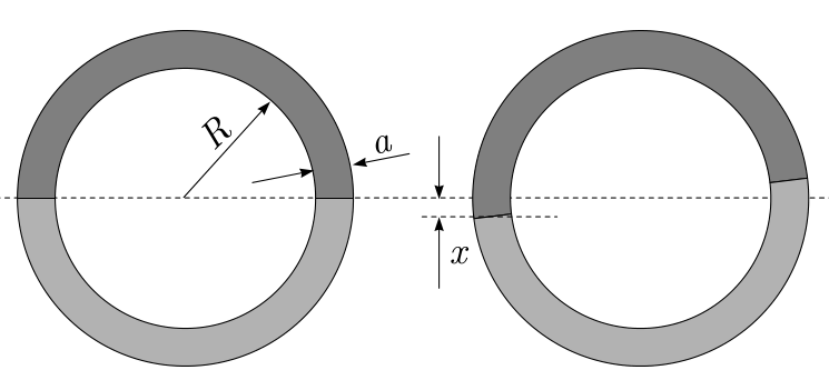
i. (1 pt) Consider a circular O-tube the lower half of which is filled with a liquid of density $ρ_{1}$ , and upper half — with a liquid of density $ρ_{2} > ρ_{1}$ , see the figure. Let the radius of the circle $R$ be much larger than the diameter of the tube $a$ (neglect the wall thickness). When the interfaces at the both sides of the O-tube are exactly at the same level (the left sketch), the system is at equilibrium. By how much will the potential energy of the system change when the interface in the left part of the tube is lowered by $x$ (as shown in the sketch on right)? Express the answer in terms of the quantities introduced above. Here and in what follows, assume that $x ≪ R$ and use the resulting approximations.

ii. (1 pt) Suppose now that the system will evolve by itself starting from the position shown in the right sketch, let us denote the speed with which the interface in the tube moves with $v = \frac{d x}{d t}$ . Express the kinetic energy of the system in terms of $v$ and the other quantities defined above.

iii. (1 pt) Show that the acceleration of the interface is proportional to its displacement $x$ by taking a time derivative of the energy conservation law, and that the displacement can grow exponentially in time so that $x$ is proportional to $e^{γ t}$ ; find $γ$ .

iv. (1 pt) Let us now substitute the O-tube with a spherical shell of radius $R$ filled with these two liquids, each of which occupies a hemispherical region inside the shell. In order to keep the interface between the liquids flat, a massless thin rigid circular membrane of radius $R$ is placed in between the liquids; the membrane can rotate frictionlessly inside the sphere, but cannot be bent. Find the instability growth rate $γ$ (defined above) if the heavier liquid occupies the upper half of the sphere.

Hint: the center of mass of a solid homogeneous hemisphere of radius $R$ is at the distance $\frac{3}{8} R$ from the sphere’s centre.

The moment of inertia of a solid sphere of mass is given by $I = \frac{2}{5} M R^{2}$ .

Small angle approximations following $sin α \approx tan α \approx α$ , $cos α \approx 1 - α^{2} /2$ can be used.

Part B. Stabilization due to surface tension (3 points)

According to the results obtained above, the Rayleigh-Taylor instability growth rate $γ$ is a decreasing function of the size $R$ of the region where the liquid starts moving. This means that small-scale perturbations of the interface shape grow faster and dominate at the initial stage of the instability. However, at very small scales, surface tension may stabilize the instability.

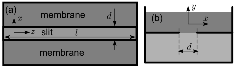
i. (1 pt) Assume that a big rectangular vessel is divided into two compartments with a thin flat membrane, the top view is shown in the figure (a) above, and a vertical cross-section with the vessel being filled with liquids — in the figure (b). The membrane has a long and narrow slit: its length $l$ is much larger than its width $d$ ( $l ≫ d$ ). The upper compartment is filled with a liquid of density $ρ_{2}$ , and the lower compartment — with a liquid of density $ρ_{1} < ρ_{2}$ . Initially, the slit is so narrow that the surface tension $σ$ which characterizes the interface between the two liquids stabilizes the Rayleigh-Taylor instability: the interface remains completely flat and horizontal. A cross-section in $x$ – $y$ -plane of this configuration is depicted in the figure (b) above, where $y$ -axis is vertical, and $z$ -axis is parallel to the longer edge of the slit. The width of the slit $d$ is increased slowly up to a certain value $d = d_{0}$ , where instabilities start developing, but the instability growth rate $γ$ remains extremely small. A special design guarantees that the deformations of the interface between the two liquids remains strictly 2-dimensional — there is no dependence on the $z$ -coordinate (this design can include, for instance, thin long rods placed onto the interface between the liquids, parallel to the slit). Sketch the new shape of the interface in $x$ – $y$ -intersection when $d = d_{0}$ and when it has become noticeably deformed due to the Rayleigh-Taylor instability.

ii. (1 pt) Consider the same setup as before, but now there are no restrictions on how the interface can be deformed, i.e. the deformation can include dependence on the $z$ -coordinate. Now, the interface becomes unstable at somewhat smaller slit width $d = d_{1}$ . Sketch the shape of the interface when $d = d_{1}$ and it has become noticeably deformed due to the Rayleigh-Taylor instability, in two intersections with planes parallel to the $x$ – $y$ plane: one at the distance $l /4$ from one end of the slit, and the other — at the distance $l /4$ from the other end of the slit.

iii. (1 pt) Express $d_{1}$ in terms of $ρ_{1}$ , $ρ_{2}$ , $σ$ , and $g$ .

Part C. Water waves (2 points)

While a heavy liquid atop of a light one is unstable, the reverse situation of a light liquid atop of a heavy one is stable, and surface shape perturbations will travel along the surface as waves. A particular case of such waves are represented by waves on the free surface of water when the light liquid (air) has a negligibly small density. If the water is deep (much deeper than the wavelength $λ$ of the waves), the speed of sinusoidal waves depends on the wavelength,

$v = g λ /2 π .$

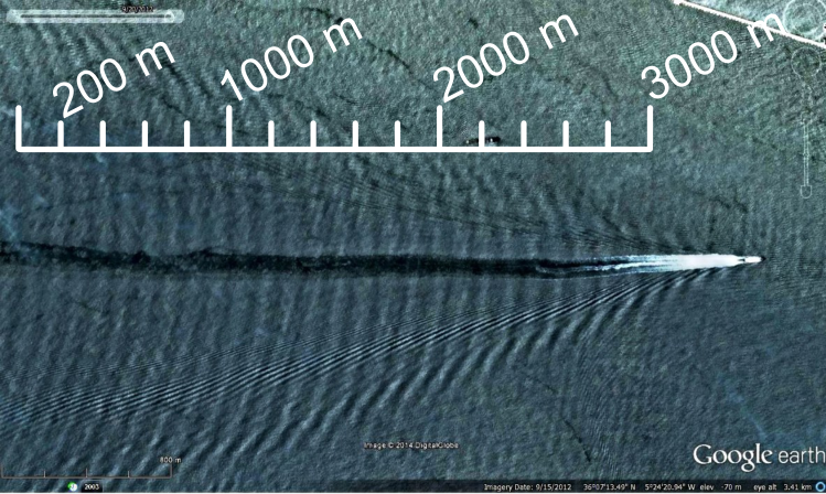
Therefore, all wave speeds are possible, including those which travel in “resonance” with the boat: the boat will always remain at the same trough or at the same crest of the wave, and will propel water resonantly, i.e. always at the same value of the phase of the wave. If there are waves which can move in a resonance with a moving object, the moving object will generate these waves — this phenomenon is known as Cherenkov radiation. Generated waves carry away energy and this results in a wave drag acting on the object. The wave drag grows rapidly with speed (proportional to the cube of the speed) and is the main limiting factor for the speed of boats. Determine the speed of the boat shown in the aerophoto below (you may take measurements from the map).

Fonte: Testo (PDF) — p.1

Topic: Fluid Mechanics, Oscillations & Waves Metodi: Energy Conservation Method, Hydrostatic Equilibrium, Differential Equations, Small-Angle Approximation Competenze: Mathematical Modeling, Physical Reasoning, Diagrammatic Reasoning Objects: Tube, Membrane

Problema T3. Instabilità di Rayleigh-Taylor (9 punti)

Lord Rayleigh mostrò nel 1883 che uno strato di liquido denso posto sopra uno strato di liquido meno denso è instabile: anche se l’interfaccia tra i due liquidi è inizialmente perfettamente piana e orizzontale, piccole perturbazioni della forma dell’interfaccia crescono esponenzialmente nel tempo: in alcuni punti il liquido pesante inizia a scendere spostando il liquido leggero sottostante, e in altri punti il liquido leggero inizia a salire — questo fenomeno è oggi noto come instabilità di Rayleigh-Taylor. Esso gioca un ruolo importante in molti campi della fisica. Per esempio, a seguito dell’esplosione di una supernova, le onde d’urto di plasma denso decelerano a causa dell‘“assorbimento” delle regioni di plasma meno denso. Questo significa che nel sistema di riferimento dell’onda d’urto in decelerazione la forza d’inerzia è diretta nel verso di propagazione dell’onda d’urto. La direzione della forza d’inerzia definisce la direzione del “basso”, cosicché il plasma più denso dell’onda d’urto appare “sopra” il plasma meno denso dello spazio interstellare. Gli stadi avanzati (non lineari) dell’instabilità sono caratterizzati da affascinanti strutture filamentose, si veda l’immagine della nebulosa del Granchio qui sotto. Nella tecnologia, l’instabilità di Rayleigh-Taylor può essere indesiderata e, per esempio, rende molto difficile realizzare il progetto della fusione a confinamento inerziale: quando inizialmente una sfera quasi perfettamente rotonda viene compressa, essa si deforma in modo irregolare — come una lattina vuota di Coca-Cola quando si cerca di comprimerla. Nel seguito costruiamo modelli matematicamente semplici per far luce sulla fisica dell’instabilità di Rayleigh–Taylor. Si assuma ovunque nel seguito che sia presente un campo gravitazionale diretto verso il basso di intensità $g$ ( $= 9.81 m/s^{2}$ ).

Parte A. Tasso di crescita dell’instabilità (4 punti)

i. (1 pt) Si consideri un tubo circolare a O la cui metà inferiore è riempita con un liquido di densità $ρ_{1}$ , e la metà superiore — con un liquido di densità $ρ_{2} > ρ_{1}$ , si veda la figura. Il raggio del cerchio $R$ sia molto maggiore del diametro del tubo $a$ (si trascuri lo spessore della parete). Quando le interfacce sui due lati del tubo a O sono esattamente allo stesso livello (schizzo a sinistra), il sistema è in equilibrio. Di quanto varia l’energia potenziale del sistema quando l’interfaccia nella parte sinistra del tubo viene abbassata di $x$ (come mostrato nello schizzo a destra)? Esprimi la risposta in termini delle grandezze introdotte sopra. Qui e nel seguito, assumi che $x ≪ R$ e usa le approssimazioni che ne derivano.

ii. (1 pt) Si supponga ora che il sistema evolva da solo a partire dalla posizione mostrata nello schizzo a destra; indichiamo con $v = \frac{d x}{d t}$ la velocità con cui si muove l’interfaccia nel tubo. Esprimi l’energia cinetica del sistema in termini di $v$ e delle altre grandezze definite sopra.

iii. (1 pt) Mostra che l’accelerazione dell’interfaccia è proporzionale al suo spostamento $x$ derivando rispetto al tempo la legge di conservazione dell’energia, e che lo spostamento può crescere esponenzialmente nel tempo in modo che $x$ sia proporzionale a $e^{γ t}$ ; trova $γ$ .

iv. (1 pt) Sostituiamo ora il tubo a O con un guscio sferico di raggio $R$ riempito con questi due liquidi, ciascuno dei quali occupa una regione emisferica all’interno del guscio. Per mantenere piana l’interfaccia tra i liquidi, tra di essi è posta una membrana circolare rigida, sottile e priva di massa, di raggio $R$ ; la membrana può ruotare senza attrito all’interno della sfera, ma non può essere piegata. Trova il tasso di crescita dell’instabilità $γ$ (definito sopra) se il liquido più pesante occupa la metà superiore della sfera.

Suggerimento: il centro di massa di un emisfero solido omogeneo di raggio $R$ si trova alla distanza $\frac{3}{8} R$ dal centro della sfera.

Il momento d’inerzia di una sfera solida di massa è dato da $I = \frac{2}{5} M R^{2}$ .

Si possono usare le approssimazioni per piccoli angoli $sin α \approx tan α \approx α$ , $cos α \approx 1 - α^{2} /2$ .

Parte B. Stabilizzazione dovuta alla tensione superficiale (3 punti)

In base ai risultati ottenuti sopra, il tasso di crescita dell’instabilità di Rayleigh-Taylor $γ$ è una funzione decrescente della dimensione $R$ della regione in cui il liquido inizia a muoversi. Questo significa che le perturbazioni della forma dell’interfaccia su piccola scala crescono più rapidamente e dominano nello stadio iniziale dell’instabilità. Tuttavia, a scale molto piccole, la tensione superficiale può stabilizzare l’instabilità.

i. (1 pt) Si assuma che un grande recipiente rettangolare sia diviso in due scomparti da una membrana piana sottile; la vista dall’alto è mostrata nella figura (a) sopra, e una sezione verticale con il recipiente riempito di liquidi — nella figura (b). La membrana presenta una fenditura lunga e stretta: la sua lunghezza $l$ è molto maggiore della sua larghezza $d$ ( $l ≫ d$ ). Lo scomparto superiore è riempito con un liquido di densità $ρ_{2}$ , e lo scomparto inferiore — con un liquido di densità $ρ_{1} < ρ_{2}$ . Inizialmente la fenditura è così stretta che la tensione superficiale $σ$ che caratterizza l’interfaccia tra i due liquidi stabilizza l’instabilità di Rayleigh-Taylor: l’interfaccia rimane completamente piana e orizzontale. Una sezione nel piano $x$ – $y$ di questa configurazione è raffigurata nella figura (b) sopra, dove l’asse $y$ è verticale e l’asse $z$ è parallelo al bordo più lungo della fenditura. La larghezza della fenditura $d$ viene aumentata lentamente fino a un certo valore $d = d_{0}$ , in corrispondenza del quale iniziano a svilupparsi instabilità, ma il tasso di crescita dell’instabilità $γ$ rimane estremamente piccolo. Un progetto particolare garantisce che le deformazioni dell’interfaccia tra i due liquidi rimangano rigorosamente bidimensionali — non c’è dipendenza dalla coordinata $z$ (questo progetto può includere, per esempio, sottili e lunghe aste poste sull’interfaccia tra i liquidi, parallele alla fenditura). Disegna la nuova forma dell’interfaccia nella sezione $x$ – $y$ quando $d = d_{0}$ e quando essa si è deformata in modo apprezzabile a causa dell’instabilità di Rayleigh-Taylor.

ii. (1 pt) Si consideri la stessa configurazione di prima, ma ora non ci sono restrizioni su come l’interfaccia può deformarsi, cioè la deformazione può includere una dipendenza dalla coordinata $z$ . Ora l’interfaccia diventa instabile per una larghezza della fenditura leggermente minore $d = d_{1}$ . Disegna la forma dell’interfaccia quando $d = d_{1}$ ed essa si è deformata in modo apprezzabile a causa dell’instabilità di Rayleigh-Taylor, in due sezioni con piani paralleli al piano $x$ – $y$ : una alla distanza $l /4$ da un’estremità della fenditura, e l’altra — alla distanza $l /4$ dall’altra estremità della fenditura.

iii. (1 pt) Esprimi $d_{1}$ in termini di $ρ_{1}$ , $ρ_{2}$ , $σ$ e $g$ .

Parte C. Onde sull’acqua (2 punti)

Mentre un liquido pesante sopra uno leggero è instabile, la situazione inversa di un liquido leggero sopra uno pesante è stabile, e le perturbazioni della forma della superficie viaggiano lungo la superficie come onde. Un caso particolare di tali onde è rappresentato dalle onde sulla superficie libera dell’acqua quando il liquido leggero (l’aria) ha una densità trascurabilmente piccola. Se l’acqua è profonda (molto più profonda della lunghezza d’onda $λ$ delle onde), la velocità delle onde sinusoidali dipende dalla lunghezza d’onda,

$v = g λ /2 π .$

Pertanto, tutte le velocità delle onde sono possibili, comprese quelle che viaggiano in “risonanza” con la barca: la barca rimarrà sempre sullo stesso cavo o sulla stessa cresta dell’onda, e spingerà l’acqua in modo risonante, cioè sempre allo stesso valore della fase dell’onda. Se esistono onde che possono muoversi in risonanza con un oggetto in movimento, l’oggetto in movimento genererà queste onde — questo fenomeno è noto come radiazione Cherenkov. Le onde generate portano via energia e ciò produce una resistenza d’onda che agisce sull’oggetto. La resistenza d’onda cresce rapidamente con la velocità (proporzionalmente al cubo della velocità) ed è il principale fattore limitante per la velocità delle barche. Determina la velocità della barca mostrata nella fotografia aerea qui sotto (puoi effettuare le misure dalla mappa).

Fonte: Testo (PDF) — p.1

Problem T3. Rayleigh-Taylor instability (9 points)

Part A. Instability growth rate (4 points)

Hint: the center of mass of a solid homogeneous hemisphere of radius $R$ is at the distance $\frac{3}{8} R$ from the sphere’s centre.

The moment of inertia of a solid sphere of mass is given by $I = \frac{2}{5} M R^{2}$ .

Small angle approximations following $sin α \approx tan α \approx α$ , $cos α \approx 1 - α^{2} /2$ can be used.

Part B. Stabilization due to surface tension (3 points)

iii. (1 pt) Express $d_{1}$ in terms of $ρ_{1}$ , $ρ_{2}$ , $σ$ , and $g$ .

Part C. Water waves (2 points)

$v = g λ /2 π .$

Fonte: Testo (PDF) — p.1

Problem E1. Magnetic properties of matter (20 points)

The aim of this experiment is to measure magnetism-related characteristics of dia- and ferromagnetic materials. To reach this goal, some other measurements are also required — e.g. measuring the diameter of the syringe needle, and the coefficient of surface tension of water.

Equipment

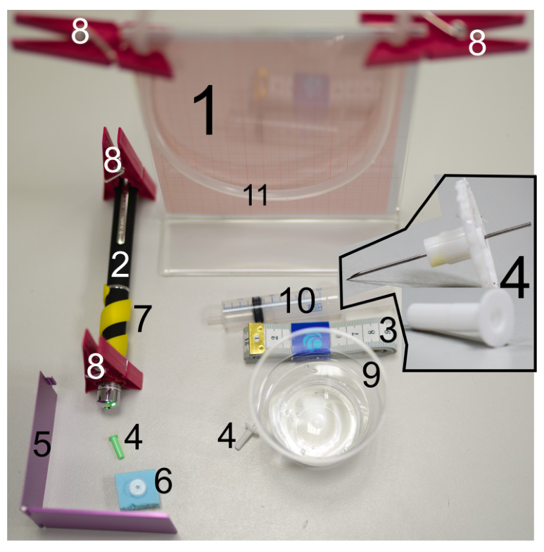
Figure 1. The following equipment is listed in figure 1:

a stand;
green laser pointer
a measuring tape;
green and white syringe needles, one end of the needle is sharp, and the other end is cut perpendicularly to its axis, see the insert in fig 1
a foldable mirror
a piece of foam
a spiral plastic fixator that keeps the laser pointer button pressed;
clothespins;
a cup with water;
a syringe;
a silicone tube.

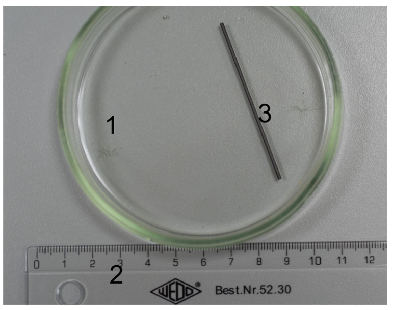
Figure 2. The following equipment is listed in figure 2:

a Petri dish;
a ruler;
a graphite bar.

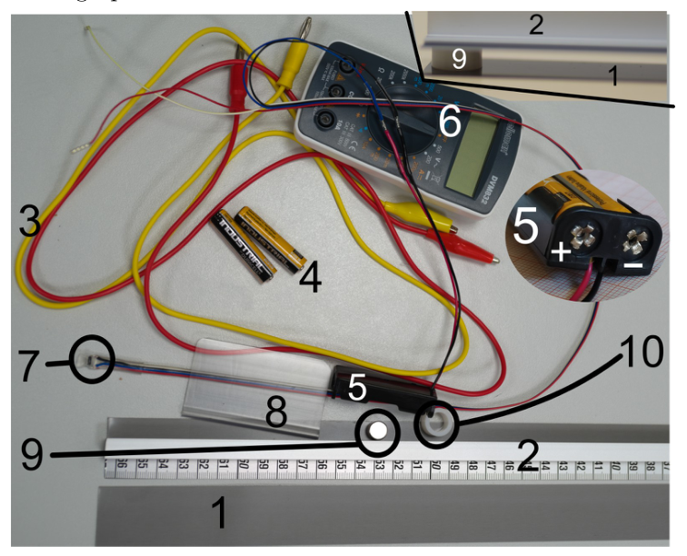
Figure 3. The following equipment is listed in figure 3:

a stand-alone ferromagnetic strip;
a ferromagnetic strip reinforced with an aluminium bar and equipped with a measuring tape;
wires with crocodile clips;
batteries;
a battery holder;
a multimeter;
a resistive magnetic field sensor;
a plastic clamp for fixing the orientation of the sensor;
a magnet;
a plastic spacer to keep the strip (2) strictly horizontal.

Not shown in the figures: a piece of polyethylene film for wrapping the magnet.

WARNINGS:

Do not bend the ferromagnet, as it will become unusable! If bent, no replacement will be provided and you will get no marks for that part.
Avoid direct or reflected laser beams hitting your eye, this can be harmful to your eye!
The syringe needles are sharp, avoid puncturing yourself!
Avoid short-circuiting the battery leads — the battery will overheat and become unusable!
Power off the multimeter and the laser when not in use, in order to conserve the batteries.

Tasks

Part A. Diameter of the syringe needle (3 points)

Determine the diameter of the syringe needles using the following procedure.

Put the syringe standing vertically onto table, with its plastic cap downside as shown in Fig 4B, install the laser with the help of the clothspins as shown in the figure, and direct the laser beam onto the needle. If the laser beam is too high (i.e. passes the needle above it), you may use the piece of foam as shown in Fig 4A (insert the sharp end of the green syringe needle into the foam so that it will stand vertically). If the laser beam is slightly too low, you may use a folded sheet of paper to raise it. If the laser runs out of battery, you may ask for a replacement. Use the mirror to increase the length of the laser beam (see Fig 4A). Measure the distance between diffraction maxima on the screen as precisely as possible (explain how you achieved the best possible accuracy). Measure the length of the light beam from the syringe needle to the screen and calculate the diameter of the needle. Wavelength of the laser beam is $λ = 532 nm$ .

Estimate the uncertainty of your result. Repeat the procedure with the white needle.

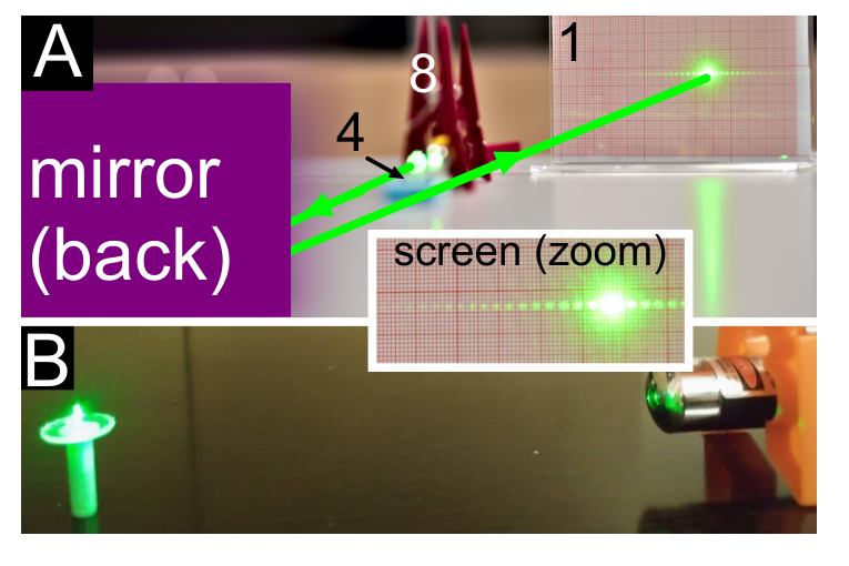
Figure 4.

Part B. Surface tension of water (4 points)

Fill the silicon tube with water — you may use the syringe (do not use the needle!) so that approximately 2/3rd of it is filled with water (adjust the amount of water as needed later); make sure that the water forms a continuous column with no air gaps. Using clamps, fix the tube from its two ends to the screen (which is now used as a stand). Insert the green syringe needle into the tube by puncturing it with the sharp end of the needle. Make sure to puncture the tube perpendicularly near its centre, so that the flat end of the needle will point vertically downwards. Depending on the height of the water column above the open end of the needle, water may or may not start slowly dripping out. If it does not drip, lower the needle by pulling the tube from its middle part downwards so that it will start approaching a V-shape. If water still does not start dripping, add more water into the tube (if even this is not enough, ask for a replacement needle).

While the water is slowly dripping from the needle, raise very slowly the needle to determine, at which height will the dripping stop, and measure the corresponding water column height (the height difference between the water level in the tube, and the lowest point of the needle).

Hint: when the tube is hanging in a U-shaped manner, the height of the water column can be adjusted by pulling the tube from its middle point into a V-shape, or raising it into a W-shape.

Make several measurements with the green needle, and repeat the whole procedure with the white needle. State your results for the critical water column heights together with the uncertainties, for the both needles. Based on your measurements, determine the coefficient of surface tension $σ$ for water, alongside its uncertainty. Density of water is $ρ_{w} = 1000 kg/m^{3}$ , free fall acceleration $g = 9.81 m/s^{2}$ .

Hints: different stages of the droplet growing from the end of the syringe needle are shown in Fig 5. Surface tension gives rise to a pressure drop over a curved water surface; in the case of a spherical surface, this pressure drop equals to $Δ p = 2 σ / r$ , where $r$ is the radius of the spherical surface.

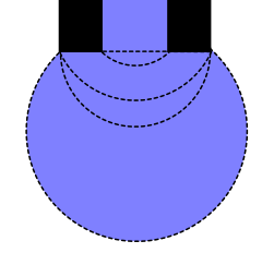
Figure 5.

Part C. Susceptibility of graphite (4 points)

Measure the diameter of the magnet and write down the result.

Fill the Petri dish with water so that the water layer depth is approximately half of the dish height. Break a tiny piece from the graphite bar and put it onto the water; it should remain floating owing to surface tension.

Fix the magnet to the syringe as shown in Fig. 6 (magnet’s axis should be parallel to the syringe) with the help of a piece of the polyethylene film. Orient the magnet approximately under 45 degrees to the horizon (so that the angle between the syringe and vertical direction equals approximately to the angle between the syringe and the horizontal plane). When you move the magnet closer to the piece of graphite, it will “swim” away due to diamagnetism. Push it towards a wall of the Petri dish. When the magnet is not too far away from the wall, for each position of the magnet, there is an equilibrium position of the graphite pebble. You need to achieve two different equilibrium configurations: (a) the magnet’s diameter and the graphite pebble form approximately an equilateral triangle; (b) the magnet’s diameter and the graphite pebble form approximately an isosceles right triangle, see Fig. 6.

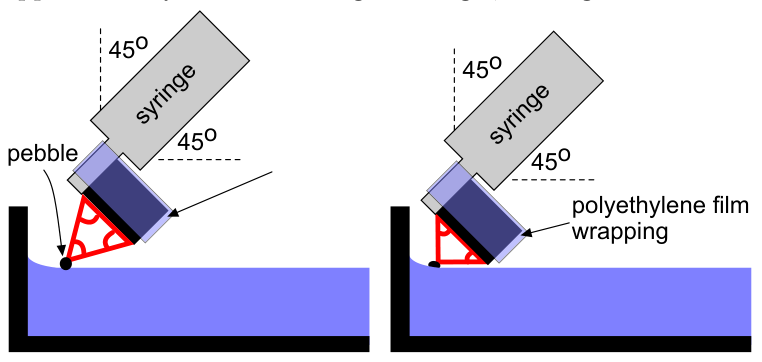
Figure 6.

Using the ruler, measure the distance between the pebble and the wall of the dish for the both configurations; repeat measurements several time to reduce uncertainty.

The pushing force exerted on the graphite pebble per unit mass of the pebble is given by the formula

$\frac{F}{m} = (∣ χ_{g} - χ_{w} ∣) \frac{1}{2 μ _{0}} \frac{d B ^{2}}{d z},$

where $χ_{g}$ and $χ_{w} = - 9.05 \times 1 0^{- 9} m^{3} / kg$ are the specific susceptibilities of the graphite and of the water (per unit mass of the material), and $\frac{1}{2 μ _{0}} \frac{d B ^{2}}{d z}$ denotes the magnetic pressure gradient.

Fig. 7 shows the water surface slope angle $α$ as a function of the horizontal displacement $x$ from the vertical wall of the dish, normalized to the characteristic length scale $σ / ρ_{w} g$ . Here $ρ_{w} = 1000 kg$ is the density of water, and $g = 9.81 m/s^{2}$ is the free fall acceleration. The graphite pebble will rest at very small angles so that the approximation $α ≪ 1$ can be used.

Fig. 8 shows the magnetic pressure gradient at the magnet’s axis as a function of distance from the flat face of the given permanent magnet.

Based on these data and your measurements from before, determine $χ_{g}$ and estimate its uncertainty.

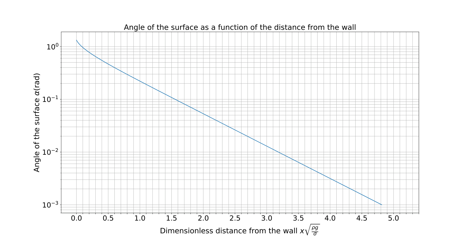
Figure 7.

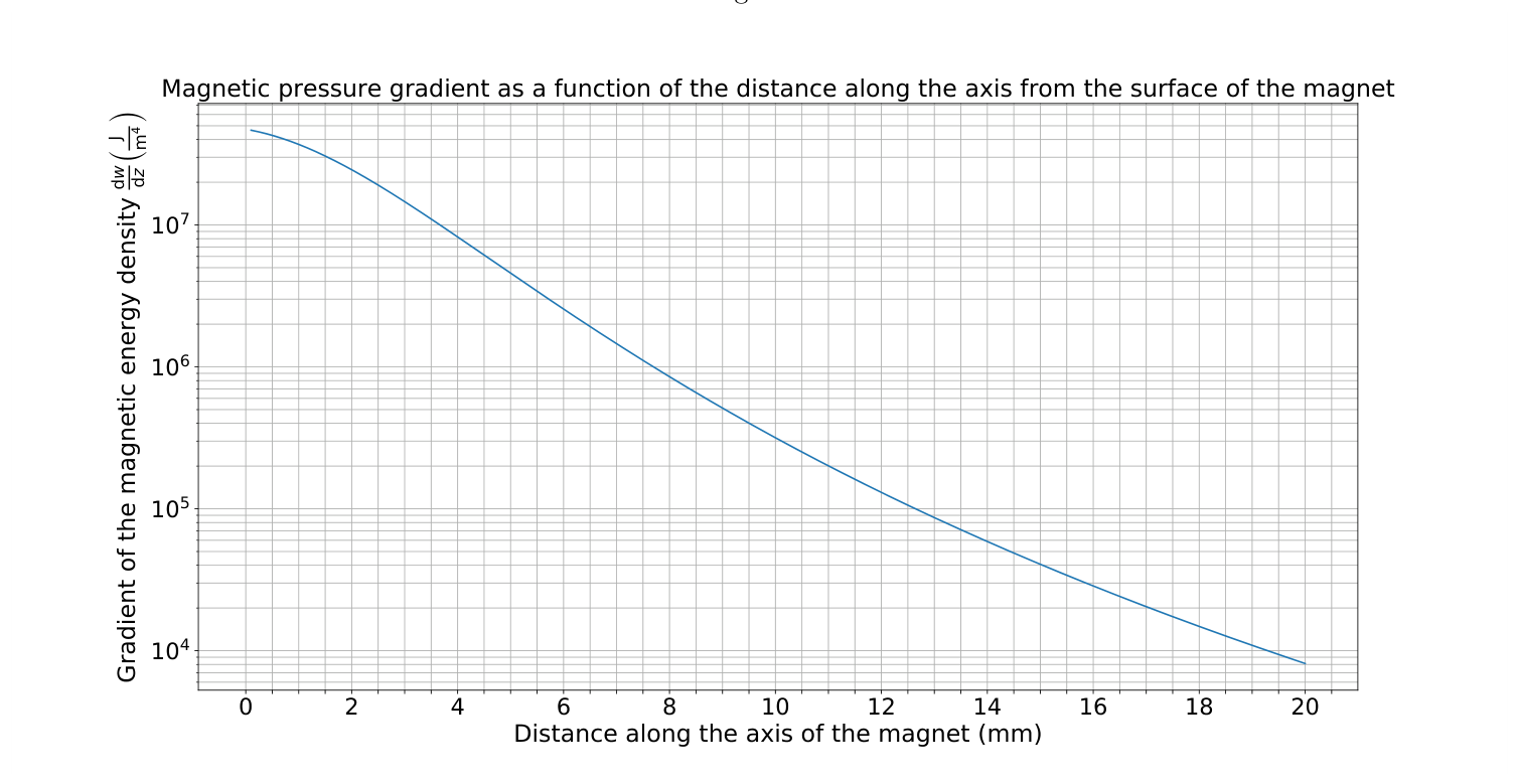
Figure 8.

Part D. Relative permeability of ferromagnetic strip (9 points)

i. (1 pt) Measure the voltage $E$ on the output leads of the battery holder using the multimeter by connecting multimeter to the leads shown as ”+” and ”−” in the insert of Fig 3 and switching it to 20 volt (DC) range. If the voltage is below 3.0 V, you may ask for replacement batteries.

Connect the blue and black wires of the magnetic sensor to the batteries in the battery holder, and the red and white wires to the multimeter. If the plastic clamp is put around the four wires near the sensor as shown if Fig 3, the sensor is kept in such a position that vertical magnetic field will be measured. Switch on the multimeter in 200 millivolt (DC) range, put the sensor onto table far away from the magnet and the ferromagnetic strips, take the reading of the multimeter $V_{0}$ , and write it down. Subtract this voltage reading from all the subsequent readings (to compensate for the zero offset of the sensor, and for the magnetic field of the Earth).

ii. (4 pts) If the battery voltage were to be exactly 3 V, each millivolt in the reading would correspond to 10 microteslas of the magnetic field strength. However, the reading is proportional to the battery voltage.

Put the stand-alone ferromagnetic strip onto table; place the magnet and the plastic cylindrical spacer onto it, as close as possible to its endpoints (see the insert of Fig 3), and the reinforced strip onto the whole assembly so that a gap of constant width is formed between the strips. Measure the magnetic field strength $B = B (z)$ between the two strips as a function of distance $z$ from the magnet-less end of the strips. Start with the farthest possible position from the magnet, with $z$ equal to a few millimeters, and use 5 cm increments. For each distance $z$ , move the sensor between the strips horizontally to find the largest possible reading. Tabulate your direct voltage readings together with the corresponding magnetic field strengths.

Theory predicts that in this configuration, the magnetic field between the strips is

$B = B_{0} cosh (z / λ),$

where

$λ = μ δ h /2$

and the hyperbolic cosine is defined as $cosh x = \frac{1}{2} (e^{x} + e^{- x})$ . Here, $δ = 0.27 mm$ stands for the strip thickness and $h$ — for the width of the gap between the two strips. This can be measured using a ruler. Based on your measurements data, draw an appropriate graph to determine the relative magnetic permeability $μ$ . Find $μ$ and estimate the uncertainty of your result.

Hints: the given expression for $B (z)$ fails due to the saturation effect if the magnetic field inside the ferromagnetic strip is too large. Calculators usually do have both cosh-function, as well as its inverse function, denoted as acosh or $cosh^{- 1}$ .

iii. (2 pts) In order to understand how the magnetic flux is distributed over the width of the strip, measure the magnetic field strength as a function of the distance $s$ from the symmetry axis of the strip for a certain fixed value of $z$ in the middle of its range; use 4 mm-increments and decrease these increments wherever appropriate. Plot the results. Comment on your results.

iv. (2 pts) Assuming that the distribution of the magnetic flux over the width of the strip is almost independent on $z$ , calculate and plot the magnetic field strength inside the ferromagnetic strip as a function of $z$ based on your measurement data (you may take additional measurements if needed). Estimate the field strength $B_{s}$ by which the magnetization of the ferromagnetic material starts becoming saturated.

Fonte: Testo (PDF) — p.1

Topic: Magnetism, Electromagnetism Metodi: Experimental Data Analysis, Interference & Diffraction Analysis, Graph Linearization, Lorentz Force Analysis Competenze: Experimental Data Analysis, Measurement & Instrumentation, Error Propagation, Graph Linearization Objects: Mirror, Magnet, Battery, Droplet

Problem E1. Magnetic properties of matter (20 points)

L’obiettivo di questo esperimento è di misurare le caratteristiche legate al magnetismo dei materiali dia- e ferromagnetic. Per raggiungere questo obiettivo, sono necessarie anche altre misure. misura il diametro della agola della siringa e il coefficiente di tensione di superficie dell’acqua.

# # Equipaggiamento

Figura 1. Le seguenti apparecchiature sono elencate in Figura 1:

a) stazione;
puntatore laser verde
a misurazione;
aghi di seringa verde e bianca, una estremità dell’ago è acuta, e l’altra estremità è tagliata perpendicolare al suo asse, vedere l’inserimento in fig. 1
un specchio pieghevole
un pezzo di schiuma
un fissatore di plastica a spirale che mantiene il pulsante laser pointer premuto;
i vestiti;
un calice con acqua;
a siringa;
un tubo di silicone.

Figura 2. Le seguenti apparecchiature sono elencate in figura 2:

a piatto di petri;
a ruotare;
- Un bar di graffiti.

Figura 3. Le seguenti apparecchiature sono elencate in figura 3:

a) una striscia ferromagnetico stand-alone;
una striscia ferromagnetico rinforzata con una barra di alluminio e equipaggiata con una cinta di misura;
i fili con clip di crocodili;
batterie;
un batterista;
a multimetro;
a sensore di campo magnetico resistivo;
un tampone di plastica per fissare l’orientamento del sensore;
a magnete;
un spazzatore di plastica per mantenere la striscia (2) strettamente orizzontale.

Non mostrato nelle cifre: un pezzo di film di polietilene per avvolgere il magnete.

**ALVORTI: **

Non piegare il ferromagnete, come sarà diventato inutilizzabile! Se è, non ci sarà alcun sostituto e non otterrai alcun marchio per quella parte.
Evita i raggi laser diretti o riflessi che colpiscono l’occhio, questo può essere dannoso per l’occhio!
Le agole della siringa sono taglienti, evita di punturarti!
Evita di short-circuiting le batterie che si superiscelano e diventano inutilizzabili!
Spegni il multimetro e il laser quando non in uso, per conservare le batterie.

Tasche

# # # # Parte A. Diametro della agola della siringa (3 punti)

Determina il diametro delle agole della siringa usando la procedura seguente.

Metti la siringa in piedi verticalmente su un tavolo, con il suo cappello in plastica a lato come mostrato in Fig. 4B, installa il laser con l’aiuto dei spins del tessuto come mostrato nella figura, e dirigi il laser beam sullo spino. Se il laser beam è troppo alto (cioè passera’ l’ago sopra di esso), si può usare il pezzo di schiuma come mostrato in Figura 4A (inserire l’estremità acuta dell’ago della siringa verde nella schiuma in modo che sia in piedi verticalmente). Se il fascio laser è leggermente troppo basso, si può usare un foglio di carta piegato per alzarlo. Se il laser si esaurisce, potresti chiedere un sostituto. Usare il mirror per aumentare la lunghezza del fascio laser (vedi figura 4A). Misurare la distanza tra la diffrazione massima sullo schermo con la massima precisione possibile (esplorar come hai raggiunto la migliore accuratezza possibile). Measure the length of the light beam from the syringe needle to the screen and calculate the diameter of the needle. L’onda del fascio laser è $λ = 532 nm$ .

Estimare l’incertezza del tuo risultato. Ripeti la procedura con l’ago bianco.

Figura 4.

Parte B. Tensione di superficie dell’acqua (4 punti)

Riempi il tubo di silicio con acqua puoi usare la siringa (non usare l’ago!) in modo che circa 2/3 di essa sia riempita con acqua (adjust the amount of water as needed later); assicurati che l’acqua formi una colonna continua senza gap di aria. Usando le prese, risolvi il tubo dalle sue due estremità allo schermo (che è ora usato come stand). Inserire l’ ago verde nella tubulazione punzionandolo con l’ estremità acuta dell’ ago. Assicurati di puncture il tubo perpendicolare vicino al suo centro, in modo che la fine piatta dell’ago punterà verticalmente verso il basso. A seconda dell’altezza della colonna d’acqua sopra l’aperto di punta dell’ago, l’acqua può o non può iniziare a scorrere lentamente. Se non goccia, abbassare l’ago tirando il tubo dalla sua parte media verso il basso in modo che inizierà ad avvicinarsi a una forma V. Se l’acqua non inizia ancora a gocciolare, aggiungere più acqua nel tubo (se anche questo non è sufficiente, chiedere un ago di sostituzione).

Mentre l’acqua è lentamente gocciolando dal ago, sollevare molto lentamente l’ago per determinare, a quale altezza si fermerà il gocciolo, e misurare la corrispondente altezza della colonna d’acqua (la differenza di altezza tra il livello dell’acqua nel tubo, e il punto più basso dell’ago).

Quando il tubo è appeso in forma di U, l’altezza della colonna d’acqua può essere regolata tirando il tubo dal suo punto medio in una forma di V o sollevandolo in una forma di W.

Fare diverse misurazioni con l’ago verde e ripetere l’intera procedura con l’ago bianco. Indicare i risultati per le altezze critiche dell’acqua colonna insieme alle incertezze, per le aghi entrambe. Basato sulle vostre misure, determinate il coefficiente di tensione di superficie $σ$ per l’acqua, oltre alla sua incertezza. Density of water is $ρ_{w} = 1000 kg/m^{3}$ , free fall acceleration $g = 9.81 m/s^{2}$ .

Infine, la dose di riserva deve essere somministrata a un livello di 0,5% di dose. La tensione di superficie dà luogo a un calo di pressione su una superficie di acqua curva; nel caso di una superficie sferica, questo calo di pressione equivale a $Δ p = 2 σ / r$ , dove $r$ è il raggio della superficie sferica.

Figura 5.

# # # # Parte C. Susceptibilità della grafite (4 punti)

Misura il diametro del magnete e scrivi il risultato.

Riempire il piatto di Petri con acqua in modo che la profondità del livello d’acqua sia circa metà dell’altezza del piatto. Sfruttare un piccolo pezzo dalla barra di graffito e metterlo sull’acqua; dovrebbe rimanere galleggiante a causa della tensione superficiale.

Fix the magnet to the syringe come mostrato in Fig. 6 (magnet’s axis should be parallel to the syringe) with the help of a piece of the polyethylene film. Orientare il magnete circa sotto i 45 gradi all’orizzonte (così che l’angolo tra la siringa e la direzione verticale sia pari circa all’angolo tra la siringa e il piano orizzontale). Quando si sposta il magnete più vicino al pezzo di grafite, si “navegerà” via a causa del diamagnetismo. Spingete verso un muro del piatto di Petri. Quando il magnete non è troppo lontano dal muro, per ogni posizione del magnete, c’è una posizione di equilibrio del pebble di graffito. You need to achieve two different equilibrium configurations: (a) il diametro del magnete e la pebble di grafite form approximately an equilateral triangle; (b) il diametro del magnete e la pebble di grafite form approximately an isosceles right triangle, see Fig. 6.

Figura 6.

Usando il ruler, misura la distanza tra il pebble e il muro del piatto per le due configurazioni; ripeta misurazioni diverse volte per ridurre l’incertezza.

La forza di spinta esercitata sul pebble grafitto per unità di massa del pebble è data dalla formula

$\frac{F}{m} = (∣ χ_{g} - χ_{w} ∣) \frac{1}{2 μ _{0}} \frac{d B ^{2}}{d z},$

dove $χ_{g}$ e $χ_{w} = - 9.05 \times 1 0^{- 9} m^{3} / kg$ sono le specificità di sensibilità della grafite e dell’acqua (per unità di massa del materiale), e $\frac{1}{2 μ _{0}} \frac{d B ^{2}}{d z}$ denota il gradiente di pressione magnetica.

Fig. 7 mostra l’angolo di pendenza della superficie dell’acqua $α$ come funzione del dislocazione orizzontale $x$ dal muro verticale del piatto, normalizzato alla scala caratteristica di lunghezza $σ / ρ_{w} g$ . Qui $ρ_{w} = 1000 kg$ è la densità di acqua, e $g = 9.81 m/s^{2}$ è l’accelerazione della caduta libera. Il graphite pebble sarà riposato a angoli molto piccoli in modo che l’approssimazione $α ≪ 1$ possa essere utilizzata.

Fig. 8 mostra il gradiente di pressione magnetica all’asse del magnete come funzione della distanza dal lato piatto del magnete permanente dato.

Basato su questi dati e sulle tue misurazioni di prima, determina $χ_{g}$ e stima la sua incertezza.

Figura 7.

Figura 8.

Parte D. Permeabilità relativa della striscia ferromagnetico (9 punti)

i. (1 pt) Measure the voltage $E$ on the output leads of the battery holder using the multimeter by connecting multimeter to the leads shown as ”+” and ”−” in the insert of Fig 3 and switching it to 20 volt (DC) range. Se la tensione è inferiore a 3,0 V, potresti chiedere batterie di sostituzione.

Connettere i fili blu e neri del sensore magnetico alle batterie del portatore della batteria, e i fili rossi e bianchi al multimetro. Se il supporto plastico è posto intorno ai quattro fili vicino al sensore come mostrato in Fig. 3, il sensore è tenuto in una posizione tale da misurare il campo magnetico verticale. Switch on the multimeter in 200 millivolt (DC) range, put the sensor onto table far away from the magnet and the ferromagnetic strips, take the reading of the multimeter $V_{0}$ , and write it down. Sottrazione di questa lettura di tensione da tutte le letture successive (per compensare il zero offset del sensore, e per il campo magnetico della Terra).

**ii. (4 pts) ** Se la batteria fosse esattamente 3 V, ogni milivolt in lettura corrisponderebbe a 10 microteslas della forza del campo magnetico. Tuttavia, la lettura è proporzionale alla tensione della batteria.

Metti la striscia ferromagnetico stand-alone su un tavolo; metti il magnete e il spazzatore cilindrico di plastica su di esso, il più vicino possibile ai suoi punti di fine (vedi l’inserimento di Figura 3), e la striscia rinforzata su tutta l’assemblea in modo che un gap di costante larghezza sia formato tra le strisce. Misurare la forza del campo magnetico $B = B (z)$ tra le due strisce come funzione di distanza $z$ dal magnete-less end delle strisce. Inizia con la posizione più lontana possibile dal magnete, con $z$ pari a pochi millimetri, e usa increments di 5 cm. For each distance $z$ , move the sensor between the strips horizontally to find the largest possible reading. Tabulate le letture di tensione diretta insieme alle corrispondenti forze del campo magnetico.

La teoria prevede che in questa configurazione, il campo magnetico tra le strisce è

$B = B_{0} cosh (z / λ),$

dove

$λ = μ δ h /2$

e il cosino iperbolico è definito come $cosh x = \frac{1}{2} (e^{x} + e^{- x})$ . Qui, $δ = 0.27 mm$ significa lo spessore della striscia e $h$ indica la larghezza del gap tra le due strisce. Questo può essere misurato usando un ruoter. Based on your measurements data, draw an appropriate graph to determine the relative magnetic permeability $μ$ . Find $μ$ and estimate the uncertainty of your result.

Infine, l’espressione data per $B (z)$ fa faillito a causa dell’effetto saturazione se il campo magnetico all’interno della striscia ferromagnetica è troppo grande. Calcolatori di solito hanno entrambe le funzioni Cosh, così come la sua funzione inversa, denotate come acosh o $cosh^{- 1}$ .

**iii. (2 pts) ** Per capire come il flusso magnetico è distribuito sulla larghezza della striscia, misurare la forza del campo magnetico come funzione della distanza $s$ dall’asse di simmetria della striscia per un certo valore fisso di $z$ nel mezzo del suo range; utilizzare 4 mm increments e diminuire questi increments ove appropriato. - Pianifica i risultati. Commento sui risultati.

**iv. (2 pts) ** Supponendo che la distribuzione del flusso magnetico sulla larghezza della striscia sia quasi indipendente su $z$ , calcolare e tracciare la forza del campo magnetico all’interno della striscia ferromagnetico come funzione di $z$ basata sui dati di misurazione (potete prendere ulteriori misurazioni se necessario). Estimare la forza di campo $B_{s}$ con cui la magnetizzazione del materiale ferromagnetico inizia a diventare saturazione.

Fonte: Testo (PDF) — p.1

Problem E1. Magnetic properties of matter (20 points)

The aim of this experiment is to measure magnetism-related characteristics of dia- and ferromagnetic materials. To achieve this goal, some other measurements are also required e.g. measuring the diameter of the syringe needle, and the coefficient of surface tension of water.

Equipment

Figure 1. The following equipment is listed in Figure 1:

a stand;
Green laser pointer
a measuring tape;
green and white syringe needles, one end of the needle is sharp, and the other end is cut perpendicular to its axis, see the insert in Fig 1
a foldable mirror
a piece of foam
a spiral plastic fixator that keeps the laser pointer button pressed;
a weight of not more than 0,5% but less than 0,5%
a cup with water;
a syringe;
A silicone tube.

Figure 2. The following equipment is listed in Figure 2:

a petri dish;
a. Rulers;
A graphite bar.

Figure 3. The following equipment is listed in Figure 3:

a stand-alone ferromagnetic strip;
a ferromagnetic strip reinforced with an aluminium bar and equipped with a measuring tape;
wires with crocodile clips;
batteries;
a battery holder;
a multimeter;
a resistive magnetic field sensor;
a plastic clamp for fixing the orientation of the sensor;
a magnet;
a plastic spacer to keep the strip (2) strictly horizontal.

Not shown in the figures: a piece of polyethylene film for wrapping the magnet.

WARNINGS:

Do not bend the ferromagnet, as it will become unusable! If bent, no replacement will be provided and you will get no marks for that part.
Avoid direct or reflected laser beams hitting your eye, this can be harmful to your eye!
The syringe needles are sharp, avoid puncturing yourself!
Avoid short-circuiting the battery leads the battery will overheat and become unusable!
Turn off the multimeter and the laser when not in use, to conserve the batteries.

Tasks

Part A. The diameter of the syringe needle (3 points)

Determine the diameter of the syringe needles using the following procedure.

Put the syringe standing vertically onto the table, with its plastic cap downside as shown in Figure 4B, install the laser with the help of the cloth spins as shown in the figure, and direct the laser beam onto the needle. If the laser beam is too high (i.e. passes the needle above it), you may use the piece of foam as shown in Figure 4A (insert the sharp end of the green syringe needle into the foam so that it will stand vertically). If the laser beam is slightly too low, you may use a folded sheet of paper to raise it. If the laser runs out of battery, you may ask for a replacement. Use the mirror to increase the length of the laser beam (see Figure 4A). Measure the distance between diffraction maxima on the screen as precisely as possible (explain how you achieved the best possible accuracy). Measure the length of the light beam from the syringe needle to the screen and calculate the diameter of the needle. Wavelength of the laser beam is $λ = 532 nm$ .

Estimate the uncertainty of your result. Repeat the procedure with the white needle.

Figure 4.

Part B. Surface tension of water (4 points)

Fill the silicon tube with water you may use the syringe (don’t use the needle!) so that approximately 2/3rd of it is filled with water (adjust the amount of water as needed later); make sure that the water forms a continuous column with no air gaps. Using clamps, fix the tube from its two ends to the screen (which is now used as a stand). Insert the green syringe needle into the tube by puncturing it with the sharp end of the needle. Make sure to puncture the tube perpendicularly near its center, so that the flat end of the needle will point vertically downwards. Depending on the height of the water column above the open end of the needle, water may or may not start dripping out slowly. If it doesn’t drip, lower the needle by pulling the tube from its middle part downwards so that it will start approaching a V-shape. If water still does not start dripping, add more water into the tube (if even this is not enough, ask for a replacement needle).

While the water is slowly dripping from the needle, raise very slowly the needle to determine, at what height will the dripping stop, and measure the corresponding water column height (the height difference between the water level in the tube, and the lowest point of the needle).

Hint: when the tube is hanging in a U-shaped manner, the height of the water column can be adjusted by pulling the tube from its middle point into a V-shape, or raising it into a W-shape.

Make several measurements with the green needle, and repeat the entire procedure with the white needle. State your results for the critical water column heights together with the uncertainties, for the both needles. Based on your measurements, determine the coefficient of surface tension $σ$ for water, alongside its uncertainty. Density of water is $ρ_{w} = 1000 kg/m^{3}$ , free fall acceleration $g = 9.81 m/s^{2}$ .

Hints: different stages of the droplet growing from the end of the syringe needle are shown in Figure 5. Surface tension gives rise to a pressure drop over a curved water surface; in the case of a spherical surface, this pressure drop equals to $Δ p = 2 σ / r$ , where $r$ is the radius of the spherical surface.

Figure 5.

Part C. Susceptibility of graphite (4 points)

Measure the diameter of the magnet and write down the result.

Fill the Petri dish with water so that the water layer depth is approximately half of the dish height. Break a tiny piece from the graphite bar and put it on the water; it should remain floating due to surface tension.

Fix the magnet to the syringe as shown in Fig. 6 (magnet’s axis should be parallel to the syringe) with the help of a piece of the polyethylene film. Orient the magnet approximately under 45 degrees to the horizon (so that the angle between the syringe and vertical direction is approximately equal to the angle between the syringe and the horizontal plane). When you move the magnet closer to the piece of graphite, it will “swim” away due to diamagnetism. Push it towards a wall of the Petri dish. When the magnet is not too far away from the wall, for each position of the magnet, there is an equilibrium position of the graphite pebble. You need to achieve two different equilibrium configurations: (a) the magnet’s diameter and the graphite pebble form approximately an equilateral triangle; (b) the magnet’s diameter and the graphite pebble form approximately an isosceles right triangle, see Fig. 6.

Figure 6.

Using the ruler, measure the distance between the pebble and the wall of the dish for the both configurations; repeat measurements several time to reduce uncertainty.

The force of pushing exerted on the graphite pebble per unit mass of the pebble is given by the formula

$\frac{F}{m} = (∣ χ_{g} - χ_{w} ∣) \frac{1}{2 μ _{0}} \frac{d B ^{2}}{d z},$

Fig. 8 shows the magnetic pressure gradient at the magnet’s axis as a function of distance from the flat face of the given permanent magnet.

Based on these data and your measurements from before, determine $χ_{g}$ and estimate its uncertainty.

Figure 7.

Figure 8.

Part D. Relative permeability of ferromagnetic strip (9 points)

Connect the blue and black wires of the magnetic sensor to the batteries in the battery holder, and the red and white wires to the multimeter. If the plastic clamp is placed around the four wires near the sensor as shown in Figure 3, the sensor is kept in such a position that vertical magnetic field will be measured. Switch on the multimeter in 200 millivolt (DC) range, put the sensor onto table far away from the magnet and the ferromagnetic strips, take the reading of the multimeter $V_{0}$ , and write it down. Subtract this voltage reading from all the subsequent readings (to compensate for the zero offset of the sensor, and for the magnetic field of the Earth).

**ii. (4 pts) ** If the battery voltage were to be exactly 3 V, each millivolt in the reading would correspond to 10 microteslas of the magnetic field strength. However, the reading is proportional to the battery voltage.

Place the magnet and the plastic cylindrical spacer on it, as close as possible to its endpoints (see the insert of Fig. 3), and the reinforced strip onto the entire assembly so that a gap of constant width is formed between the strips. Measure the magnetic field strength $B = B (z)$ between the two strips as a function of distance $z$ from the magnet-less end of the strips. Start with the farthest possible position from the magnet, with $z$ equal to a few millimeters, and use 5 cm increments. For each distance $z$ , move the sensor between the strips horizontally to find the largest possible reading. Tabulate your direct voltage readings together with the corresponding magnetic field strengths.

The theory predicts that in this configuration, the magnetic field between the strips is

$B = B_{0} cosh (z / λ),$

where

$λ = μ δ h /2$

and the hyperbolic cosine is defined as $cosh x = \frac{1}{2} (e^{x} + e^{- x})$ . Here, $δ = 0.27 mm$ stands for the strip thickness and $h$ for the width of the gap between the two strips. This can be measured using a ruler. Based on your measurements data, draw an appropriate graph to determine the relative magnetic permeability $μ$ . Find $μ$ and estimate the uncertainty of your result.

Hints: the given expression for $B (z)$ fails due to the saturation effect if the magnetic field inside the ferromagnetic strip is too large. Calculators usually do have both cosh function, as well as its inverse function, denoted as acosh or $cosh^{- 1}$ .

**iii. (2 pts) ** To understand how the magnetic flux is distributed over the width of the strip, measure the magnetic field strength as a function of the distance $s$ from the symmetry axis of the strip for a certain fixed value of $z$ in the middle of its range; use 4 mm increments and decrease these increments where appropriate. Plot the results. Comment on your results.

**iv. (2 pts) ** Assuming that the distribution of the magnetic flux over the width of the strip is almost independent on $z$ , calculate and plot the magnetic field strength inside the ferromagnetic strip as a function of $z$ based on your measurement data (you may take additional measurements if needed). Estimate the field strength $B_{s}$ by which the magnetization of the ferromagnetic material starts to become saturated.

Fonte: Testo (PDF) — p.1

Raccolta Gare di Fisica

Esplora

GPhO 2019

Part A. Zero-g flight (3 points)

Part B. Glass of water in weightlessness (3 points)

Part C. Sharpshooter on geostationary orbit (4 points)

Parte A. Zero-g flight (3 punti)

Parte B. Glass of water in weightlessness (3 punti)

Parte C. Sharpshooter in orbita geostationaria (4 punti)

Part A. Zero-g flight (3 points)

Part B. Glass of water in weightlessness (3 points)

Part C. Sharpshooter on geostationary orbit (4 points)

Part A. General considerations (0.5 points)

Part B. Tokamak (2.5 points)

Part C. Cold fusion (3.5 points)

Part D. Inertial confinement fusion (4.5 points)

Parte A. Considerazioni generali (0,5 punti)

Parte B. Tokamak (2.5 punti)

Parte C. Fusione a freddo (3,5 punti)

Parte D. Fusione a confinamento inertio (4.5 punti)

Part A. General considerations (0.5 points)

Part B. The following points are added:

Part C. Cold fusion (3.5 points)

Part D. Inertial confinement fusion (4.5 points)

Part A. Instability growth rate (4 points)

Part B. Stabilization due to surface tension (3 points)

Part C. Water waves (2 points)

Parte A. Tasso di crescita dell’instabilità (4 punti)

Parte B. Stabilizzazione dovuta alla tensione superficiale (3 punti)

Parte C. Onde sull’acqua (2 punti)

Part A. Instability growth rate (4 points)

Part B. Stabilization due to surface tension (3 points)

Part C. Water waves (2 points)

Equipment

Tasks

Part A. Diameter of the syringe needle (3 points)

Part B. Surface tension of water (4 points)

Part C. Susceptibility of graphite (4 points)

Part D. Relative permeability of ferromagnetic strip (9 points)

# # Equipaggiamento

Tasche

# # # # Parte A. Diametro della agola della siringa (3 punti)

Parte B. Tensione di superficie dell’acqua (4 punti)

# # # # Parte C. Susceptibilità della grafite (4 punti)

Parte D. Permeabilità relativa della striscia ferromagnetico (9 punti)

Equipment

Tasks

Part A. The diameter of the syringe needle (3 points)

Part B. Surface tension of water (4 points)

Part C. Susceptibility of graphite (4 points)

Part D. Relative permeability of ferromagnetic strip (9 points)

Vista grafico

Indice