IZhO 2019

Problem 1 (10.0 points)

Theoretical competition — 11 January 2019 (XV IZhO). The theoretical competition lasts 4 hours; there are three questions.

This problem consists of three independent parts.

Problem 1A (4.0 points)

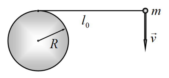
A vertical cylinder of radius $R$ is fixed on a smooth horizontal surface. A thread is tightly wound on the cylinder, the free end of which is $l_0$ long and attached to a small puck of mass $m$. The puck is initially given a horizontal velocity $v$, which is perpendicular to the thread (see figure). How long will it take for the thread to be torn up if the maximum tension force it can withstand is $T$.

Problem 1B (3.0 points)

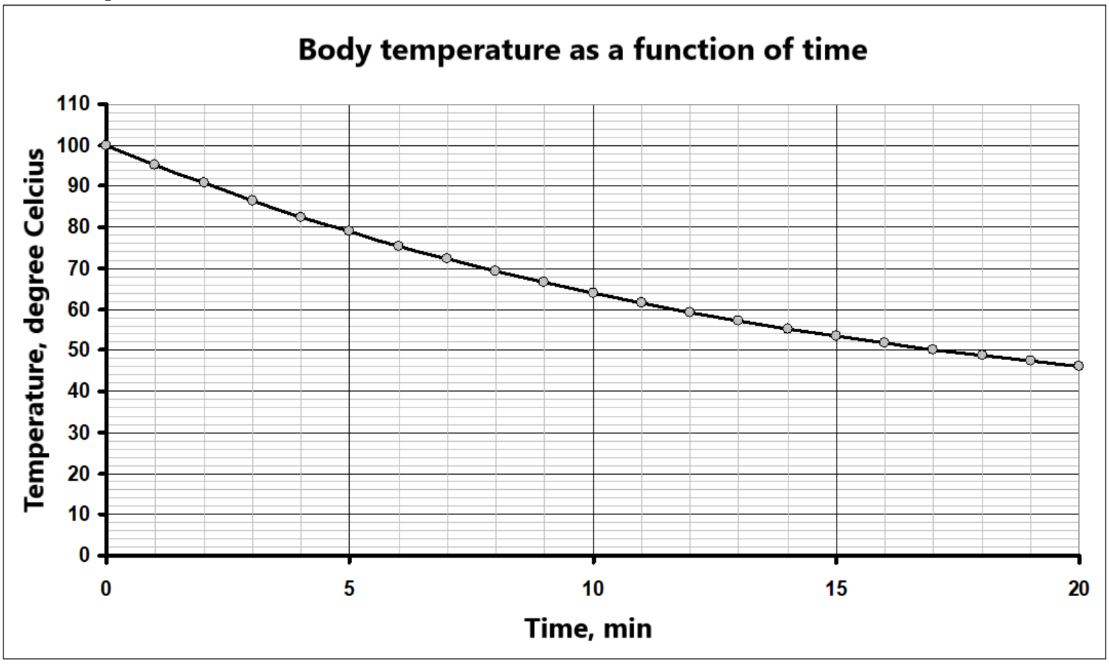
A body cools in the air so that the rate of heat transfer is proportional to the temperature difference between the body and the air. The graph below shows the dependence of the body temperature on time. Find the air temperature.

Problem 1C (3.0 points)

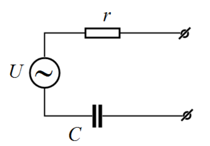
The equivalent circuit of a real source of alternating voltage of frequency $\omega =1.00\cdot 10^3{\mathrm{s}}^{-1}$ consists of an ideal voltage source with the amplitude $U=15.0\mathrm{V}$, of a resistor with the resistance $r=2019$ Ohm and of a capacitor with the capacitance $C=100\mu \mathrm{F}$. Different circuits of resistors, capacitors and coils can be connected to the source as a load. Propose a load circuit, which assures maximum of the generated heat output in the load itself. Draw schematically your load circuit and evaluate parameters of its elements. If you have found several solutions, provide the simplest one. Find also the maximum power, which can be generated in a load.

Problema 1 (10,0 punti)

Competizione teorica — 11 gennaio 2019 (XV IZhO). La competizione teorica dura 4 ore; ci sono tre domande.

Questo problema è composto da tre parti indipendenti.

Problema 1A (4,0 punti)

Un cilindro verticale di raggio $R$ è fissato su una superficie orizzontale liscia. Su di esso è avvolto strettamente un filo la cui estremità libera ha lunghezza $l_0$ ed è collegata a un piccolo dischetto di massa $m$. Inizialmente, al dischetto viene data una velocità orizzontale $v$, perpendicolare al filo (vedi figura). Quanto tempo ci vorrà perché il filo si rompa, se la massima forza di tensione che può sopportare è $T$?

Problema 1B (3,0 punti)

Un corpo si raffredda nell’aria in modo tale che la rapidità dello scambio di calore sia proporzionale alla differenza di temperatura tra il corpo e l’aria. Il grafico sottostante mostra la dipendenza della temperatura del corpo nel tempo. Determinare la temperatura dell’aria.

Problema 1C (3,0 punti)

Il circuito equivalente di una sorgente reale di tensione alternata la cui frequenza è $\omega =1,00\cdot 10^3{\mathrm{s}}^{-1}$ è costituito da una sorgente ideale di tensione con ampiezza $U=15,0\mathrm{V}$, da un resistore la cui resistenza è $r=2019$ Ohm e da un condensatore la cui capacità è $C=100\mu \mathrm{F}$. Diversi circuiti composti da resistori, condensatori e bobine possono essere collegati alla sorgente come carico. Proporre un circuito di carico che assicuri la massima potenza termica sviluppata nel carico stesso. Disegnare schematicamente il circuito di carico e stimare i parametri dei suoi elementi. Se si trovano più soluzioni, indicare la più semplice. Trovare anche la potenza massima che può essere sviluppata nel carico.

Problem 2. Conductors in an electric field (10.0 points)

When a conductor is placed in a constant external electric field, electric charges appear on its surface. This phenomenon is called an electrostatic induction, and the charges themselves are then called induced. This phenomenon is explained by a large number of free charge carriers in the conductor, usually electrons, which can move freely inside.

The distribution of the induced charges for a conductor of an arbitrary shape can be quite complex, but the following statements hold:

1. The electric field strength inside the conductor is exactly zero;
2. The electric field strength near the surface of the conductor is directed along the surface normal;
3. The induced charges are only located on the conductor surface;
4. All of the conductor points have the same electric potential.

In this problem, we consider several methods for calculating electric fields in the presence of conductors and apply them to a specific physical situation. Consider the vacuum permittivity ${\epsilon }_0$ known.

Conductive ball and point charge

A conducting ball of radius $R$ is grounded and a point-like charge $q$ is placed at a distance $l$ from it. In this case, in accordance with the foregoing, induced charges appear on the ball surface, which distort the electric field of the point-like charge $q$. The image method is applicable to this situation, whose essence is described as follows. The electric field outside the ball can be represented as a superposition of the field of the point-like charge $q$ and the field of some fictitious point-like charge $Q$ located somewhere inside the ball at a distance $a$ from its center and on the line connecting the point-like charge $q$ to the ball center. To evaluate the total electric field, we make use of the Cartesian coordinate system on the plane shown in the figure below. This is quite enough, since the system has axial symmetry.

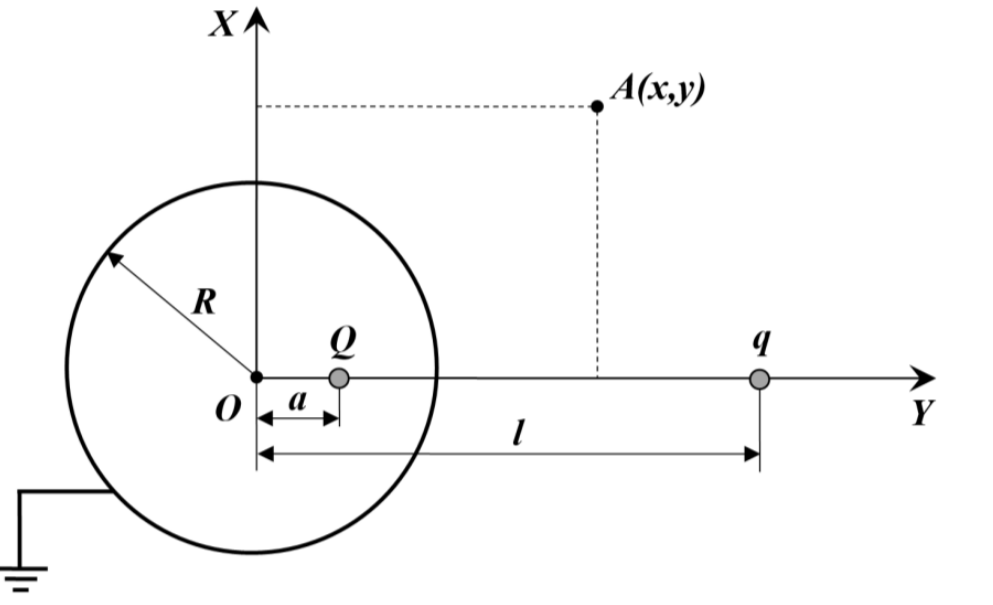
2.1 Calculate the electric field potential at an arbitrary point $A$ with coordinates $(x,y)$ lying outside the ball. Express your answer in terms of $q,Q,l,a,x,y,{\epsilon }_0$.

2.2 Using the above expression, evaluate the electric field potential on the ball surface. Express your answer in terms of $q,Q,l,a,x,R,{\epsilon }_0$.

2.3 Using your answer from 2.2, find the charge $Q$ and the distance $a$, expressing them in terms of $q,l,R$.

2.4 Calculate the work $A$ that needs to be done on the point-like charge $q$ in order to very slowly move it to infinity. Express your answer in terms of $q,l,R,{\epsilon }_0$.

2.5 Find the interaction energy $W$ of the induced charges with one another and express it in terms of $q,l,R,{\epsilon }_0$.

Conductive ball in a uniform electric field

A conducting ball of radius $R$ is placed in an external uniform electric field of strength $E_0$. In this case, the field of induced electric charges can be represented as a superposition of the field of two fictitious uniformly charged balls of the same radius $R$ located at a very small distance $a\ll R$ from each other. The net charge of these two balls is, of course, zero due to the charge conservation law, so one of them can be assumed to be charged with the bulk charge density $\rho$, whereas the other is to be charged with the bulk charge density $-\rho$.

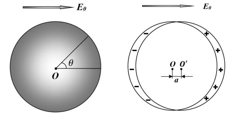
2.6 Calculate the electric field strength $E_{\rho }$ inside a uniformly charged ball with the bulk charge density $\rho$ at a distance $r$ from its center. Express your answer in terms of $\rho ,r,{\epsilon }_0$.

2.7 Calculate the electric field strength at the intersection of two fictitious balls mentioned above. Express your answer in terms of $\rho ,a,{\epsilon }_0$.

2.8 Find the surface density of the induced charges $\sigma$ as a function of the angle $\theta$ shown in the figure above. Express your answer in terms of $E_0,\theta ,{\epsilon }_0$.

2.9 Find the electric field $E$ outside the ball and just near its surface point, characterized by the angle $\theta$. Express your answer in terms of $E_0,\theta$.

Conductive ball and charged ring

A thin ring of radius $R$ is charged uniformly along its length by a charge $q$. An uncharged small conducting ball of radius $r$ and mass $m$ can slide without friction along the long non-conducting needle, coinciding with the axis of the ring.

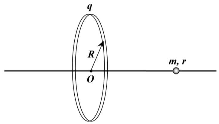
2.10 Calculate the frequency $\omega$ of small oscillations of the ball near its equilibrium position on the needle. Express your answer in terms of $q,R,r,m,{\epsilon }_0$.

2.11 The ball is initially located at the ring center and is at rest. Find the work $A$, which must be done to very slowly push the ball along the needle to infinity. Express your answer in terms of $q,R,r,{\epsilon }_0$.

Problema 2. Conduttori in un campo elettrico (10,0 punti)

Quando un conduttore viene posto in un campo elettrico esterno costante, sulla sua superficie appaiono cariche elettriche. Questo fenomeno è chiamato induzione elettrostatica, e le cariche stesse vengono definite indotte. Tale fenomeno si spiega con la presenza di un gran numero di portatori di carica liberi all’interno del conduttore, solitamente elettroni, i quali possono muoversi liberamente.

La distribuzione delle cariche indotte su un conduttore di forma arbitraria può essere piuttosto complessa, ma valgono le seguenti affermazioni:

1. L’intensità del campo elettrico all’interno del conduttore è esattamente zero;
2. L’intensità del campo elettrico vicino alla superficie del conduttore è diretta lungo la normale della superficie stessa;
3. Le cariche indotte si trovano esclusivamente sulla superficie del conduttore;
4. Tutti i punti del conduttore presentano lo stesso potenziale elettrico.

In questo problema consideriamo diversi metodi per calcolare i campi elettrici in presenza di conduttori e li applichiamo a una situazione fisica specifica. Si consideri nota la costante dielettrica del vuoto ${\epsilon }_0$.

Sfera conduttiva e carica puntiforme

Una sfera conduttrice di raggio $R$ è collegata alla terra e una carica puntiforme $q$ viene posta a una distanza $l$ da essa. In questo caso, come già accennato in precedenza, sulla superficie della sfera si formano cariche indotte che alterano il campo elettrico generato dalla carica puntiforme $q$. Per analizzare questa situazione è applicabile il metodo delle immagini, la cui essenza può essere descritta come segue: il campo elettrico esterno alla sfera può essere rappresentato come sovrapposizione del campo generato dalla carica puntiforme $q$ e di quello di una carica fittizia anch’essa puntiforme, denominata $Q$, posizionata all’interno della sfera a una distanza $a$ dal suo centro e lungo la linea che collega il punto in cui si trova la carica $q$ al centro stesso della sfera. Per calcolare il campo elettrico totale, utilizziamo il sistema di coordinate cartesiane nel piano rappresentato nella figura sottostante; tale sistema è sufficiente, poiché la situazione presenta simmetria assiale.

2.1 Calcolare il potenziale del campo elettrico in un punto qualsiasi $A$ le cui coordinate sono $(x,y)$ e che si trova all’esterno della sfera. Esprimere la risposta in termini di $q,Q,l,a,x,y,{\epsilon }_0$.

2.2 Utilizzando l’espressione ottenuta in 2.1, calcolare il potenziale del campo elettrico sulla superficie della sfera. Esprimere la risposta in termini di $q,Q,l,a,x,R,{\epsilon }_0$.

2.3 Utilizzando la risposta ottenuta in 2.2, determinare la carica $Q$ e la distanza $a$, esprimendole in termini di $q,l,R$.

2.4 Calcolare il lavoro $A$ necessario per spostare molto lentamente la carica puntiforme $q$ fino a l’infinito. Esprimere la risposta in termini di $q,l,R,{\epsilon }_0$.

2.5 Determinare l’energia di interazione $W$ delle cariche indotte tra loro ed esprimerla in termini di $q,l,R,{\epsilon }_0$.

Sfera conduttrice in un campo elettrico uniforme

Una sfera conduttrice di raggio $R$ viene posta in un campo elettrico esterno uniforme di intensità $E_0$. In questo caso, il campo delle cariche elettriche indotte può essere rappresentato come sovrapposizione dei campi di due sfere fittizie cariche uniformemente, dello stesso raggio $R$, poste a una distanza molto piccola $a\ll R$ l’una dall’altra. La carica netta di queste due sfere è, naturalmente, zero in base alla legge di conservazione della carica; pertanto, si può assumere che una delle due sia carica con la densità $\rho$ e l’altra con la densità $-\rho$.

2.6 Calcolare l’intensità del campo elettrico $E_{\rho }$ all’interno di una sfera carica uniformemente, la cui densità di carica volumetrica è $\rho$, a una distanza $r$ dal suo centro. Esprimere la risposta in termini di $\rho ,r,{\epsilon }_0$.

2.7 Calcolare l’intensità del campo elettrico nella regione di intersezione delle due sfere fittizie descritte sopra. Esprimere la risposta in termini di $\rho ,a,{\epsilon }_0$.

2.8 Determinare la densità di carica superficiale indotta $\sigma$ in funzione dell’angolo $\theta$ indicato nella figura sopra. Esprimere la risposta in termini di $E_0,\theta ,{\epsilon }_0$.

2.9 Calcolare il campo elettrico $E$ all’esterno della sfera, in prossimità del suo punto di superficie caratterizzato dall’angolo $\theta$. Esprimere la risposta in termini di $E_0,\theta$.

Sfera conduttrice e anello carico

Un sottile anello di raggio $R$ è caricato uniformemente lungo tutta la sua lunghezza con una carica $q$. Una piccola sfera conduttrice non carica, di raggio $r$ e massa $m$, può scorrere senza attrito lungo un lungo ago non conduttore che coincide con l’asse dell’anello.

2.10 Calcolare la frequenza $\omega$ delle piccole oscillazioni della sfera vicino alla sua posizione di equilibrio sull’ago. Esprimere la risposta in termini di $q,R,r,m,{\epsilon }_0$.

2.11 La sfera si trova inizialmente al centro dell’anello ed è ferma. Determinare il lavoro $A$ che deve essere compiuto per spingere molto lentamente la sfera lungo l’ago fino all’infinito. Esprimere la risposta in termini di $q,R,r,{\epsilon }_0$.

Problem 3. Laser (10.0 points)

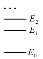
According to quantum theory, a molecule can only be found in certain states characterized by discrete energy values $E_0,E_1,E_2,\dots$. These states are represented by horizontal segments on the vertical energy scale and are numbered in order of increasing energy, starting from 0. In the absence of external influence, the molecule is found in the state with the number 0 and the lowest possible energy $E_0$. This state is then called a ground state, and the rest are then called excited states. The molecule can be driven from one energy state to another by absorbing or emitting light quanta, i.e. photons. The intensity of the light flux is characterized everywhere below by the density of the photon flux $I$, i.e. the number of photons passing perpendicularly through the unit area per unit of time, the dimension of this quantity is obviously equal to $[I]={\mathrm{m}}^{-2}\cdot {\mathrm{s}}^{-1}$.

For further consideration, it is necessary to take into account the following processes that take place when the light flux passes through a medium.

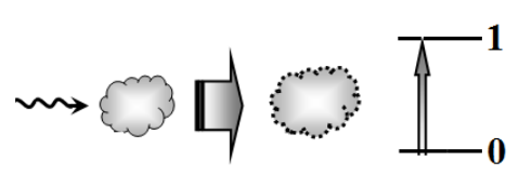
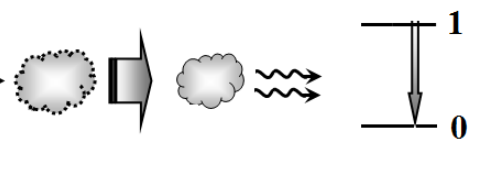
Absorption. If a molecule is found in the ground state 0, then it can absorb a photon and be raised to the excited state 1. Such a transition is possible if the photon energy is equal to the difference between the energies of the excited and ground states, $h{\nu }_{01}=E_1-E_0$, where ${\nu }_{01}$ is the photon frequency and $h=6.63\cdot 10^{-34}\mathrm{J}\cdot \mathrm{s}$ stands for the Planck constant. If $N_0$ molecules are found in the ground state 0, then the number of molecules $dN$ that have absorbed photons and have been elevated to the excited state in a very short time interval $dt$ is equal to

$dN=I{\sigma }_{01}{N}_{0}dt,(1)$

where the quantity ${\sigma }_{01}$ is called the absorption cross section and is determined by the properties of the molecules.

Stimulated emission. If a molecule is found in the excited state 1, then under the influence of a photon with the frequency ${\nu }_{01}$, it can be forced to move to the ground state 0 with the emission of another photon that is completely identical to the first one and propagates in the same direction, has the same energy and polarization. The number of such transitions $dN$ for a very small time interval $dt$ is described by the formula similar to formula (1) as

$dN=I{\sigma }_{10}{N}_{1}dt,(2)$

where $N_1$ denotes the number of molecules in the excited state 1 with energy $E_1$, and ${\sigma }_{10}$ signifies the cross section of the stimulated emission.

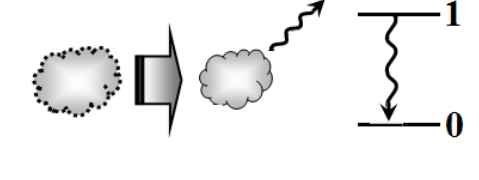
Spontaneous emission. A molecule in the excited state can spontaneously drop to its ground state with the emission of a photon. In contrast to the stimulated emission, the direction of emission and the polarization of the photon are both random, and the energy can slightly vary, i.e. the spontaneous emission cannot contribute to an increase in the light flux. The number of spontaneous transitions $dN$ from the excited state 1 to the ground state 0 for a very small time interval $dt$ is written as

$dN=A{N}_{1}dt=\frac{1}{\tau }{N}_{1}dt,(3)$

where $N_1$ still designates the number of molecules in the excited state 1 with energy $E_1$, $A$ is the transition probability or the Einstein coefficient, and its inverse value $\tau =A^{-1}$ is referred to as the lifetime of the excited state.

To describe each state $k$ of the molecule, it is convenient to use not the total number $N_k$ of molecules in the state, but its reduced value divided by the total number of molecules $N$ in the medium

$n_k=\frac{N_k}{N},(4)$

This value is called the population of the state. For populations, the normalizing condition is satisfied: the sum of the populations of all the states of the molecules is equal to unity, i.e.

$n_0+n_1+n_2+\dots =1.(5)$

If the number of molecules in a certain excited state exceeds the number of molecules in the ground state, then this state of the medium is called the population inversion, and the emitted radiation may prevail over absorption, which results in an increase in the intensity of the light flux propagating in such a medium. This phenomenon is used in optical quantum light generators, called lasers. The population inversion is conventionally created using an external energy source, called pumping. In this problem, we consider the operation of an optically pumped laser, when the population inversion is generated by an external light flux. Unlike this pumping light flux, the laser light flux is monochromatic, coherent, polarized and narrowly directed.

Population inversion: two-level system

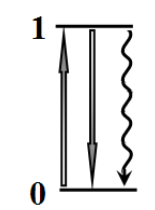
Consider a medium that is subject to monochromatic pumping light flux $I_0$. The incident light flux leads to transitions of molecules only between two states, i.e. the ground state 0 and the excited state 1. The absorption ${\sigma }_{01}$ and stimulated emission ${\sigma }_{10}$ cross sections are equal, i.e. ${\sigma }_{10}={\sigma }_{01}=\sigma$ and the lifetime in the excited state is found to be $\tau$.

3.1 Write down an equation describing the change in the population of the excited state 1 over time, i.e. express the derivative $d{n}_1/dt$ in terms of $n_1$, $I_0$, $\sigma$ and $\tau$.

3.2 Find the population of the excited state and the difference of the populations between the excited and ground states under steady conditions as functions of the pumping light flux $I_0$. Express your answer in terms of the parameter $I_0\sigma \tau$.

3.3 Is it possible to achieve an amplification of the laser light flux in this case?

Population inversion: three-level system

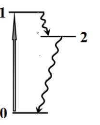
Let three states of the molecule be involved in possible transitions: the ground state 0 and the two excited states 1, 2. Under the action of the pumping light flux $I_0$, the molecule can be raised from the ground state 0 to the first excited state 1. The absorption cross section of this transition is equal to $\sigma$. As a result of intramolecular relaxation, the molecule that has resided in state 1 almost instantly drops to the lower energy state 2, whose lifetime is $\tau$. In this case, assume that the stimulated emission is completely absent.

3.4 Write down an equation describing the change in the population $n_2$ of the excited state 2 over time.

3.5 Find the population ${\bar{n}}_2$ of the excited state 2 and the population difference $({\bar{n}}_2-{\bar{n}}_0)$ of the excited and the ground states under steady conditions as functions of the pumping light flux $I_0$. Express your answer in terms of the parameter $I_0\sigma \tau$.

3.6 At what minimum value of the parameter $I_0\sigma \tau$ is it possible to amplify the laser light flux with the frequency equal to the frequency of the transition $2\to 0$?

Population inversion: four-level system

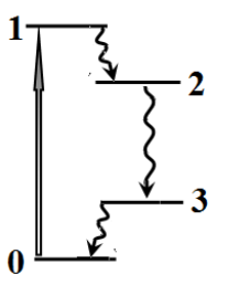
Let four states of the molecule be involved in possible transitions. Under the action of the pumping light flux $I_0$, the molecule can be raised from the ground state 0 to the first excited state 1. The absorption cross section of this transition is equal to $\sigma$. As a result of intramolecular relaxation, the molecule that has resided in state 1 almost instantly drops to the lower energy state 2, whose lifetime is $\tau$. From this state, the molecule undergoes a transition to the intermediate state 3, which results in the emission of a photon. In this case, assume that the stimulated emission is completely absent. As a result of intramolecular relaxation, the molecule that has fallen into state 3 almost instantly drops to the ground energy state 0.

3.7 At what minimum value of the parameter $I_0\sigma \tau$ is it possible to amplify the laser light flux with the frequency equal to the frequency of the transition $2\to 3$?

Resonator

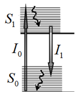
The four-level system is usually implemented in dye solutions. Dyes consist of complex molecules with multiple energy states. Therefore, the possible energy states are grouped into bands: the ground state band $S_0$ contains an almost continuous spectrum of sub-levels, and the same is true for the first excited state band $S_1$. Thus, there are two bands of possible states. The absorption of the pumping light flux $I_0$ leads to transitions from the sublevels of the ground state band $S_0$ to different sublevels of the excited state band $S_1$. Transitions between the sub-levels of state 1 occur almost instantaneously, so the stimulated emission of the laser light flux $I_1$ occurs at lower frequencies, and the stimulated emission due to the pumping light flux $I_0$ can be neglected. In the approximation described, it is sufficient to know the population of the ground and excited state bands. Rhodamine 6G is used as a dye, for which: the absorption cross section in the transition $S_0\to S_1$ is ${\sigma }_A=3,90\cdot 10^{-16}\mathrm{c}{\mathrm{m}}^2$; the stimulated emission cross section $S_1\to S_0$ is ${\sigma }_E=2,20\cdot 10^{-16}\mathrm{c}{\mathrm{m}}^2$; the lifetime of the molecule in the state $S_1$ is $\tau =4,20\cdot 10^{-9}\mathrm{s}$.

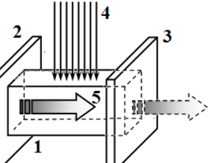
To generate light, cuvette 1 with the solution of rhodamine 6G is placed between two parallel mirrors 2 and 3, thus forming a resonator. The solution is excited by a uniform pumping light flux 4 of intensity $I_0$, whose frequency strictly corresponds to the maximum absorption of the solution. The pumping light flux 4 is directed perpendicular to the axis of the resonator and fully illuminates the entire cell. The intensity of this flux, of course, decreases as it passes through the solution; however, for carrying out our estimations, consider $I_0$ constant in the entire bulk of the resonator, assuming it to be averaged over the solution volume. The laser light flux 5 generated in the resonator propagates along the resonator axis, and its amplification occurs due to multiple reflections from the resonator mirrors. Consider mirror 2 fully reflective, and the second mirror 3 translucent with the reflectance $\rho$. The absorption of light in the mirrors, the solvent-body, as well as the scattering of light and other losses can be completely ignored. The resonator has the following parameters: the cuvette length is $l=3,00\mathrm{cm}$; the rhodamine 6G concentration is $\gamma =1.30\cdot 10^{16}\mathrm{c}{\mathrm{m}}^{-3}$; the reflection coefficient of the translucent mirror is $\rho =0,90$; the refractive index of the solution of rhodamine 6G is $r=1,50$. The speed of light is denoted as $c=3,00\cdot 10^{10}cm/s$.

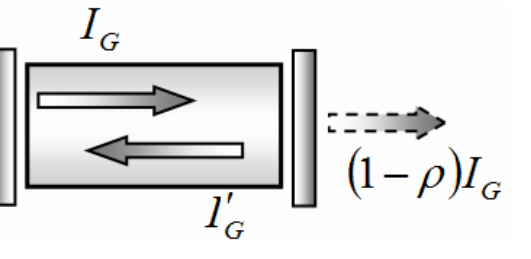
For a simplified description of the laser light flux propagating along the resonator axis, one can consider the intensity of the light fluxes averaged over the length of the resonator. We denote the average intensity of the laser light flux propagating to the translucent mirror as $I_G$, and the intensity of the laser light flux propagating in the opposite direction as $I_G^{\prime }$. Since the transmittance of mirror 3 is small, then we can assume that the average intensities of these fluxes be approximately equal $I_G\approx I_G^{\prime }$.

3.8 Let a laser light flux $I_G$ be created in the resonator. Show that in the absence of absorption and stimulated emission, the change in the intensity of the laser flux over time is described by the equation

$\frac{d{I}_G}{dt}=-\frac{1}{T}{I}_G,(6)$

where $T$ stands for the so-called photon lifetime in the resonator. Express the parameter $T$ in terms of the parameters of the resonator. Calculate its numerical value.

3.9 Show that in the absence of the photon losses through mirror 3, the laser light flux variation over time obeys the following equation

$\frac{d{I}_G}{dt}=Kn{I}_G,(7)$

where $n$ designates the population of the excited state of rhodamine 6G, and $K$ is the resonator gain. Express the resonator gain $K$ in terms of the parameters of the resonator and the stimulated emission cross section ${\sigma }_E$ of rhodamine 6G. Calculate its numerical value.

Stationary generation mode

In this part, we assume that the pumping light flux is constant and does not depend on time. In the stationary mode, all quantities remain constant: the population of the excited state and the laser light flux. Assume that the population of the excited state is low, i.e. $n\ll 1$.

3.10 Write down a set of equations describing the change in the population $\frac{dn}{dt}$ of the excited state and the laser light flux $\frac{d{I}_G}{dt}$ in the resonator.

3.11 Obtain the formula and calculate a minimum (threshold) value $n_{th}$ of the population of the excited state at which the amplification (generation) of laser light in the resonator occurs. Express it in terms of the parameters of the resonator $K,T$.

3.12 Derive the formula and calculate a minimum (threshold) value of the pumping light flux $I_{0,th}$ at which the laser light amplification in the resonator starts. Let the wavelength of the pumping light flux be $\lambda =520\mathrm{nm}$. Calculate the pumping flux in energetic units of $W/c{\mathrm{m}}^2$.

3.13 Find the laser flux at the output of the resonator as a function of the pumping light flux $I_0$, and express it in terms of the ratio $\eta =I_0/I_{0,th}$, which is called the threshold overrun, and the characteristics of molecules. Draw a graph of the laser flux at the output of the resonator as a function $\eta$.

3.14 Find the quantum output $f=N_E/N_A$, i.e. the ratio of the number of photons $N_E$ leaving the resonator per unit of time to the number of photons $N_A$ absorbed in the resonator per the same unit of time as a function of the parameter $\eta$.

Mathematical hint for the theoretical competition. You may need to know the following integrals: $\int \frac{dx}{ax+b}=\frac{1}{a}\ln |ax+b|,$ $\int x^{n}dx=\frac{x^{n+1}}{n+1},\text{where }n\text{ is an integer number.}$

Problema 3. Laser (10,0 punti)

Secondo la teoria quantistica, una molecola può trovarsi soltanto in determinati stati caratterizzati da valori discreti di energia $E_0,E_1,E_2,\dots$. Questi stati sono rappresentati da segmenti orizzontali sulla scala energetica verticale e sono numerati in ordine crescente di energia, a partire da 0. In assenza di influenze esterne, la molecola si trova nello stato con il numero 0 e l’energia più bassa possibile, $E_0$. Questo stato viene chiamato stato fondamentale, mentre gli altri vengono definiti stati eccitati. La molecola può passare da uno stato energetico all’altro assorbendo o emettendo quanti di luce, cioè fotoni. L’intensità del flusso luminoso è caratterizzata dalla densità di flusso di fotoni $I$, ovvero dal numero di fotoni che attraversano perpendicolarmente un’unità di superficie in un’unità di tempo; la dimensione di questa grandezza è chiaramente $[I]={\mathrm{m}}^{-2}\cdot {\mathrm{s}}^{-1}$.

Per ulteriori considerazioni, è necessario prendere in considerazione i seguenti processi che avvengono quando il flusso luminoso attraversa un mezzo.

Assorbimento. Se una molecola si trova nello stato fondamentale 0, può assorbire un fotone e passare allo stato eccitato 1. Tale transizione è possibile se l’energia del fotone è uguale alla differenza tra le energie degli stati eccitato e fondamentale, $h{\nu }_{01}=E_1-E_0$, dove ${\nu }_{01}$ è la frequenza del fotone e $h=6,63\cdot 10^{-34}\mathrm{J}\cdot \mathrm{s}$ rappresenta la costante di Planck. Se ci sono $N_0$ molecole nello stato fondamentale 0, il numero di molecole $dN$ che hanno assorbito fotoni e passato allo stato eccitato in un intervallo di tempo molto breve $dt$ è uguale a

$dN=I{\sigma }_{01}{N}_{0}dt,(1)$

dove la quantità ${\sigma }_{01}$ è chiamata sezione d’assorbimento e viene determinata dalle proprietà delle molecole.

Emissione stimolata. Se una molecola si trova nello stato eccitato 1, allora, sotto l’influenza di un fotone con frequenza ${\nu }_{01}$, può essere indotta a passare allo stato fondamentale 0 attraverso l’emissione di un altro fotone identico al primo, che si propaga nella stessa direzione e possiede la stessa energia e polarizzazione. Il numero di tali transizioni, $dN$, in un intervallo di tempo molto breve $dt$, è descritto da una formula simile alla formula (1).

$dN=I{\sigma }_{10}{N}_{1}dt,(2)$

dove $N_1$ indica il numero di molecole nello stato eccitato 1, con energia $E_1$, e ${\sigma }_{10}$ rappresenta la sezione trasversale dell’emissione stimolata.

Emissione spontanea. Una molecola nello stato eccitato può passare spontaneamente allo stato fondamentale emettendo un fotone. A differenza dell’emissione stimolata, sia la direzione di emissione che la polarizzazione del fotone sono casuali, e l’energia emessa può variare leggermente; pertanto, l’emissione spontanea non può contribuire all’aumento del flusso luminoso. Il numero di transizioni spontanee $dN$ dallo stato eccitato 1 allo stato fondamentale 0 in un intervallo di tempo molto breve $dt$ si scrive

$dN=A{N}_{1}dt=\frac{1}{\tau }{N}_{1}dt,(3)$

dove $N_1$ indica ancora il numero di molecole nello stato eccitato 1 con energia $E_1$, $A$ rappresenta la probabilità di transizione o il coefficiente di Einstein; il suo valore inverso, $\tau =A^{-1}$, è detto tempo di vita dello stato eccitato.

Per descrivere ciascuno stato $k$ della molecola, è conveniente utilizzare non il numero totale $N_k$ di molecole in quello stato, ma il suo valore ridotto diviso per il numero totale di molecole $N$ presenti nel mezzo

$n_k=\frac{N_k}{N},(4)$

Questo valore viene definito “popolazione dello stato”. Per quanto riguarda le popolazioni, viene soddisfatta la condizione di normalizzazione: la somma delle popolazioni di tutti gli stati delle molecole è uguale a uno, cioè

$n_0+n_1+n_2+\dots =1.(5)$

Se il numero di molecole in uno stato eccitato supera quello di molecole nello stato fondamentale, allora questo stato del mezzo viene definito “inversione di popolazione”. In tal caso, la radiazione emessa può prevalere sull’assorbimento, con conseguente aumento dell’intensità del flusso luminoso che si propaga in tale mezzo. Questo fenomeno viene sfruttato nei generatori quantistici ottici di luce, chiamati laser. L’inversione di popolazione viene solitamente generata utilizzando una fonte esterna di energia, detta pompaggio. In questo problema consideriamo il funzionamento di un laser a pompaggio ottico, in cui l’inversione di popolazione è generata da un flusso luminoso esterno. A differenza di questo flusso di pompaggio, il flusso luminoso laser è monocromatico, coerente, polarizzato e strettamente direzionato.

Inversione di popolazione: sistema a due livelli

Si consideri un mezzo soggetto a un flusso luminoso monocromatico di pompaggio pari a $I_0$. Il flusso luminoso incidente provoca transizioni delle molecole soltanto tra due stati, ovvero lo stato fondamentale 0 e lo stato eccitato 1. Le sezioni d’assorbimento ${\sigma }_{01}$ e di emissione stimolata ${\sigma }_{10}$ sono uguali, cioè ${\sigma }_{10}={\sigma }_{01}=\sigma$, e il tempo di vita nello stato eccitato è pari a $\tau$.

3.1 Scrivere un’equazione che descriva la variazione nel tempo della popolazione dello stato eccitato 1, cioè esprimere la derivata $d{n}_1/dt$ in termini di $n_1$, $I_0$, $\sigma$ e $\tau$.

3.2 Trovare, in condizioni stazionarie, la popolazione dello stato eccitato e la differenza di popolazione tra stato eccitato e stato fondamentale in funzione del flusso luminoso di pompaggio $I_0$. Esprimere i risultati in termini del parametro $I_0\sigma \tau$.

3.3 È possibile ottenere un’amplificazione del flusso luminoso laser in questo caso?

Inversione di popolazione: sistema a tre livelli

Siano tre stati della molecola coinvolti nelle possibili transizioni: lo stato fondamentale 0 e i due stati eccitati 1, 2. Sotto l’azione del flusso luminoso di pompaggio $I_0$, la molecola può essere elevata dallo stato fondamentale 0 al primo stato eccitato 1. La sezione d’assorbimento di questa transizione è uguale a $\sigma$. A seguito di processi di rilassamento intramolecolare, la molecola che si trova nello stato 1 scende quasi immediatamente allo stato a energia più bassa, lo stato 2, il cui tempo di vita è $\tau$. In questo caso, si assuma che l’emissione stimolata sia completamente assente.

3.4 Scrivere un’equazione che descriva la variazione nel tempo della popolazione $n_2$ dello stato eccitato 2.

3.5 Trovare la popolazione ${\bar{n}}_2$ dello stato eccitato 2 e la differenza di popolazione tra stato eccitato e stato fondamentale, $({\bar{n}}_2-{\bar{n}}_0)$, in condizioni stazionarie, in funzione del flusso luminoso di pompaggio $I_0$. Esprimere i risultati in termini del parametro $I_0\sigma \tau$.

3.6 A quale valore minimo del parametro $I_0\sigma \tau$ è possibile amplificare il flusso luminoso laser la cui frequenza corrisponde alla frequenza della transizione $2\to 0$?

Inversione di popolazione: sistema a quattro livelli

Siano quattro stati della molecola coinvolti nelle possibili transizioni. Sotto l’azione del flusso luminoso di pompaggio $I_0$, la molecola può essere elevata dallo stato fondamentale 0 al primo stato eccitato 1. La sezione d’assorbimento di questa transizione è uguale a $\sigma$. A seguito di processi di rilassamento intramolecolare, la molecola che si trova nello stato 1 scende quasi immediatamente allo stato a energia inferiore 2, il cui tempo di vita è $\tau$. Da questo stato, la molecola subisce una transizione verso lo stato intermedio 3, che comporta l’emissione di un fotone. In questo caso, si assuma che l’emissione stimolata sia completamente assente. Ancora a seguito di processi di rilassamento intramolecolare, la molecola che è passata allo stato 3 scende quasi immediatamente allo stato fondamentale 0.

3.7 A quale valore minimo del parametro $I_0\sigma \tau$ è possibile amplificare il flusso luminoso del laser, la cui frequenza è uguale alla frequenza della transizione $2\to 3$?

Risonatore

Il sistema a quattro livelli viene solitamente realizzato in soluzioni di coloranti. I coloranti sono costituiti da molecole complesse con diversi stati energetici; pertanto, questi stati vengono raggruppati in “bande”. La banda dello stato fondamentale $S_0$ contiene uno spettro quasi continuo di sottolivelli, e lo stesso vale per la prima banda dello stato eccitato $S_1$. Esistono quindi due bande di stati possibili. L’assorbimento del flusso luminoso di pompaggio $I_0$ provoca transizioni dai sottolivelli della banda $S_0$ a diversi sottolivelli della banda $S_1$. Le transizioni tra i sottolivelli dello stato $S_1$ avvengono quasi istantaneamente; pertanto, l’emissione stimolata del flusso luminoso laser $I_1$ si verifica a frequenze più basse, e l’emissione stimolata dovuta al flusso luminoso di pompaggio $I_0$ può essere trascurata. Nell’approssimazione descritta, è sufficiente conoscere la popolazione delle molecole nelle bande dello stato fondamentale e dello stato eccitato. Come colorante viene utilizzata la rodamina 6G; per questa sostanza: la sezione d’assorbimento nella transizione $S_0\to S_1$ è ${\sigma }_A=3,90\cdot 10^{-16}\mathrm{c}{\mathrm{m}}^2$; la sezione d’emissione stimolata nella transizione $S_1\to S_0$ è ${\sigma }_E=2,20\cdot 10^{-16}\mathrm{c}{\mathrm{m}}^2$; il tempo di vita della molecola nello stato $S_1$ è $\tau =4,20\cdot 10^{-9}\mathrm{s}$.

Per generare luce, la cuvetta 1 contenente la soluzione di rodamina 6G viene posta tra due specchi paralleli, 2 e 3, formando così un risonatore. La soluzione viene eccitata da un flusso luminoso di pompaggio uniforme, 4, di intensità $I_0$, la cui frequenza corrisponde esattamente al massimo assorbimento della soluzione stessa. Il flusso luminoso di pompaggio è diretto perpendicolarmente all’asse del risonatore e illumina completamente l’intera cella. L’intensità di questo flusso diminuisce naturalmente durante il suo passaggio attraverso la soluzione; tuttavia, per i calcoli che stiamo effettuando, consideriamo $I_0$ costante in tutto il volume del risonatore, assumendolo mediato sul volume della soluzione. Il flusso luminoso laser, 5, generato all’interno del risonatore si propaga lungo l’asse di questo e la sua amplificazione avviene grazie alle molteplici riflessioni sui suoi specchi. Si consideri lo specchio 2 completamente riflettente, mentre lo specchio 3 è traslucido, con un coefficiente di riflessione pari a $\rho$. L’assorbimento della luce negli specchi, nel solvente e le altre perdite legate alla diffusione della luce possono essere completamente ignorate. I parametri del risonatore sono i seguenti: la lunghezza della cuvetta è $l=3,00\mathrm{cm}$; la concentrazione di rodamina 6G nella soluzione è $\gamma =1,30\cdot 10^{16}\mathrm{c}{\mathrm{m}}^{-3}$; il coefficiente di riflessione dello specchio traslucido è $\rho =0,90$; l’indice di rifrazione della soluzione di rodamina 6G è $r=1,50$. La velocità della luce è indicata con $c=3,00\cdot 10^{10}cm/s$.

Per una descrizione semplificata del flusso di luce laser che si propaga lungo l’asse del risonatore, si può considerare l’intensità del flusso di luce media lungo la lunghezza del risonatore. Denotiamo con $I_G$ l’intensità media del flusso di luce laser che si dirige verso lo specchio traslucido, e con $I_G^{\prime }$ l’intensità del flusso di luce laser che si propaga nella direzione opposta. Poiché la trasmissione dello specchio 3 è bassa, possiamo assumere che queste intensità medie siano approssimativamente uguali, ovvero $I_G\approx I_G^{\prime }$.

3.8 Si supponga che nel risonatore sia presente un flusso di luce laser $I_G$. Dimostrare che, in assenza di assorbimento ed emissione stimolata, la variazione nel tempo dell’intensità del flusso laser è descritta dall’equazione

$\frac{d{I}_G}{dt}=-\frac{1}{T}{I}_G,(6)$

dove $T$ è il cosiddetto tempo di vita del fotone nel risonatore. Esprimere il parametro $T$ in termini dei parametri del risonatore e calcolarne il valore numerico.

3.9 Dimostrare che, in assenza di perdite di fotoni attraverso lo specchio 3, la variazione nel flusso di luce laser nel tempo segue l’equazione

$\frac{d{I}_G}{dt}=Kn{I}_G,(7)$

dove $n$ indica la popolazione dello stato eccitato della rodamina 6G e $K$ è il guadagno del risonatore. Esprimere il guadagno $K$ in termini dei parametri del risonatore e della sezione trasversale di emissione stimolata ${\sigma }_E$ della rodamina 6G. Calcolarne il valore numerico.

Regime di generazione stazionario

In questa parte, assumiamo che il flusso di luce di pompaggio sia costante e non dipenda dal tempo. Nel regime stazionario, tutte le grandezze rimangono costanti: la popolazione dello stato eccitato e il flusso di luce laser. Assumiamo che la popolazione dello stato eccitato sia bassa, cioè $n\ll 1$.

3.10 Scrivere un sistema di equazioni che descrivano il cambiamento nella popolazione dello stato eccitato $\frac{dn}{dt}$ e nel flusso di luce laser $\frac{d{I}_G}{dt}$ all’interno del risonatore.

3.11 Ricavare la formula e calcolare il valore minimo (di soglia) $n_{th}$ della popolazione dello stato eccitato al quale avviene l’amplificazione (generazione) della luce laser nel risonatore. Esprimerlo in termini dei parametri del risonatore $K,T$.

3.12 Ricavare la formula e calcolare il valore minimo (di soglia) del flusso di luce di pompaggio $I_{0,th}$ al quale inizia l’amplificazione della luce laser nel risonatore. Si supponga che la lunghezza d’onda del flusso di luce di pompaggio sia $\lambda =520\mathrm{nm}$. Calcolare il flusso di pompaggio in unità energetiche di $W/c{\mathrm{m}}^2$.

3.13 Determinare il flusso laser in uscita dal risonatore in funzione del flusso di luce di pompaggio $I_0$, ed esprimerlo in termini del rapporto $\eta =I_0/I_{0,th}$, noto come «superamento della soglia», nonché delle caratteristiche molecolari. Tracciare un grafico del flusso laser in uscita dal risonatore in funzione di $\eta$.

3.14 Determinare il rendimento quantico $f=N_E/N_A$, cioè il rapporto tra il numero di fotoni $N_E$ che lasciano il risonatore per unità di tempo e il numero di fotoni $N_A$ assorbiti nel risonatore nello stesso lasso di tempo, in funzione del parametro $\eta$.