IZhO 2023

Problem 1 (10.0 points)

Theoretical competition — February 2, 2023 (XIX IZhO).

This problem consists of three independent parts.

Problem 1.1 (4.0 points)

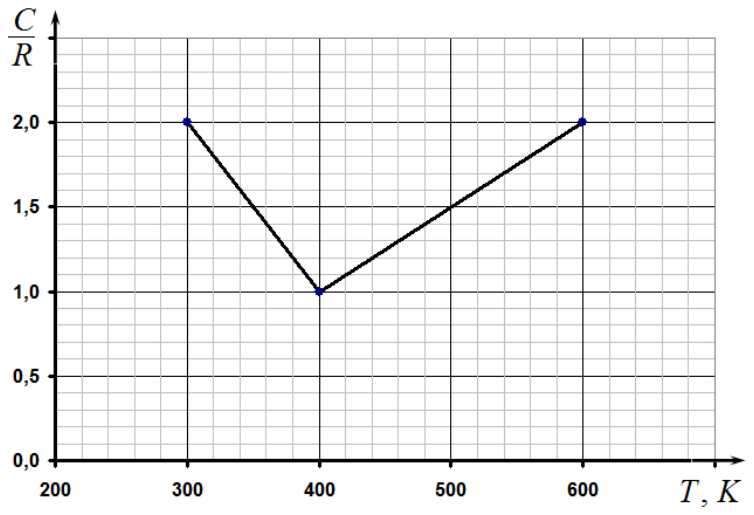
One mole of an ideal monatomic gas, located in the cylinder under the piston, is quasi-statically heated from the temperature $T_1=300\text{K}$ to $T_2=600\text{K}$, changing its volume in such a way that the dependence of the heat capacity $C$ of the gas on its temperature has the form shown in the figure below. Find the work done on the gas from the state in which the graph of its volume versus temperature reaches a local maximum, to the state in which the same graph reaches a local minimum. Express your answer in joules assuming that $R=8.31\text{J/K}$ is the universal gas constant.

Problem 1.2 (3.0 points)

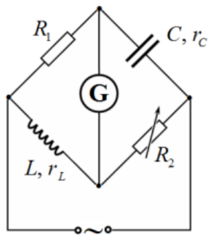
The figure on the right shows an AC bridge circuit. The resistance $R_1=2.5\text{k}\Omega$, the inductance $L=1\text{H}$, the resistance of the inductance $r_L=1\Omega$ are all known. At the frequency of the alternating sinusoidal voltage $\nu =100\text{Hz}$, the balance of the bridge occurs at $R_2=800\Omega$. It turns out that when the frequency of the alternating current is doubled, the balance of the bridge is not violated. Find the leakage resistance $r_C$ of the capacitor and its capacitance $C$.

Problem 1.3 (4.0 points)

The Nobel Prize in Physics for 2019 was awarded to the Swiss astronomers M. Major and D. Quelo for the discovery of non-luminous satellite planets (exoplanets) around stars. Consider the planet Jupiter in our solar system as an exoplanet for the Sun. The orbital period of Jupiter is $T_J=11.9$ year at a mass of $M_J=1.90\cdot 10^{27}\text{kg}$, while the mass of the Sun is equal to $M_S=1.99\cdot 10^{30}\text{kg}$. Consider also known the speed of the Earth on its orbit $v_E=29.8\text{km/s}$, and assume that the orbits of all planets are circular. Let an observation be carried out by a spectrometer located far away from outside the solar system so that the observer is in the plane of motion of the Sun–Jupiter system. Find the minimum resolution of the spectrometer $R_{min}$, which allows one to positively detect the presence of the massive exoplanet Jupiter near the Sun. Consider the speed of light to be $c=2.99\cdot 10^8\text{m/s}$.

Note: The resolution of a spectrometer is its ability to distinguish between two closely spaced spectral lines, which is characterized by a dimensionless parameter $R=\lambda /\Delta \lambda$, where $\Delta \lambda$ denotes the smallest difference between the wavelengths of two lines still recorded as separate by the instrument, and $\lambda$ stands for the average wavelength of those two resolvable lines.

Topic: Thermodynamics, Circuits, Gravitation Metodi: First Law of Thermodynamics, Kirchhoff’s Laws, Newton’s Law of Gravitation Competenze: Mathematical Modeling, Estimation & Approximation

Problema 1 (10,0 punti)

Prova teorica – 2 febbraio 2023 (XIX IZhO).

Questo problema è composto da tre parti indipendenti.

Problema 1.1 (4,0 punti)

Una mole di un gas monatomico ideale, situato all’interno di un cilindro sotto un pistone, viene riscaldata in modo quasi statico dalla temperatura $T_1=300\text{K}$ a $T_2=600\text{K}$, e il suo volume varia in modo tale che la dipendenza della capacità termica $C$ del gas rispetto alla sua temperatura assuma la forma indicata nella figura sottostante. Calcolare il lavoro compiuto sul gas dallo stato in cui il grafico del suo volume in funzione della temperatura raggiunge un massimo locale, fino allo stato in cui lo stesso grafico raggiunge un minimo locale. Esprimere la risposta in joule, assumendo che $R=8,31\text{J/K}$ sia la costante universale dei gas.

Problema 1.2 (3,0 punti)

La figura a destra mostra un circuito a ponte in corrente alternata. La resistenza $R_1=2,5\text{k}\Omega$, l’induttanza $L=1\text{H}$ e la resistenza dell’induttanza $r_L=1\Omega$ sono tutte note. Alla frequenza della tensione sinusoidale alternata $\nu =100\text{Hz}$, il ponte raggiunge l’equilibrio quando $R_2=800\Omega$. Si scopre che, quando la frequenza della corrente alternata viene raddoppiata, l’equilibrio del ponte non viene alterato. Determinare la resistenza di dispersione $r_C$ del condensatore e la sua capacità $C$.

Problema 1.3 (4,0 punti)

Il Premio Nobel per la Fisica del 2019 è stato assegnato agli astronomi svizzeri M. Major e D. Quelo per la scoperta di pianeti satelliti non luminosi (esopianeti) in orbita attorno a stelle. Consideriamo il pianeta Giove nel nostro sistema solare come un esopianeta attorno al Sole. Il periodo orbitale di Giove è $T_J=11,9$ anni e la sua massa è $M_J=1,90\cdot 10^{27}\text{kg}$, mentre la massa del Sole è $M_S=1,99\cdot 10^{30}\text{kg}$. Si conosce inoltre la velocità della Terra sulla sua orbita, $v_E=29,8\text{km/s}$, e si assume che tutte le orbite dei pianeti siano circolari. Si supponga che un’osservazione venga effettuata da uno spettrometro situato lontano, fuori dal sistema solare, con l’osservatore nel piano di movimento del sistema Sole-Giove. Determinare la risoluzione minima dello spettrometro $R_{min}$, necessaria per rilevare con certezza la presenza dell’esopianeta Giove vicino al Sole. Si consideri che la velocità della luce sia $c=2,99\cdot 10^8\text{m/s}$.

Nota: La risoluzione di uno spettrometro è la sua capacità di distinguere due linee spettrali vicine tra loro, e viene caratterizzata da un parametro adimensionale $R=\lambda /\Delta \lambda$, dove $\Delta \lambda$ indica la minima differenza di lunghezza d’onda tra due linee che lo strumento riesce comunque a registrare separatamente, mentre $\lambda$ rappresenta la lunghezza d’onda media di queste due linee distinguibili.

Problem 2. Fermi acceleration (10.0 points)

Cosmic rays contain extremely high energy particles. A possible mechanism for the appearance of such particles is called Fermi acceleration.

Fermi acceleration is a stochastic mechanism for the acceleration that charged particles experience when they are repeatedly reflected, usually by magnetic mirrors. In this problem, we consider the main ideas underlying this paradoxical, at first glance, phenomenon.

Why are there more oncoming cars than overtaking cars?

On a motorway with three lanes A, B, C, cars move at a constant speed in one direction: along the central lane B, a car moves at a speed of $v=90\text{km/h}$; cars move along lane A at speeds $v-\Delta v=80\text{km/h}$; cars move along lane C at speeds $v+\Delta v=100\text{km/h}$. The distance between cars is the same on each of lanes A and C, the number of cars per unit of lane length for each of them is $n=5.0{\text{km}}^{-1}$.

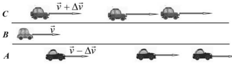
Consider the car moving in lane B.

2.1 Calculate how many cars $N_1$ in lane A overtake the car B within the time period of $t=1.0\text{min}$, as well as the time ${\tau }_1$ between two consecutive overtakes.

2.2 Calculate how many cars $N_2$ in lane C overtake the car in lane B within the time period of $t=1.0\text{min}$, as well as the time ${\tau }_2$ between two consecutive overtakes.

Now let the car move in lane B towards the cars moving in lanes A and C. The speeds of all cars and their density on each lane remain the same.

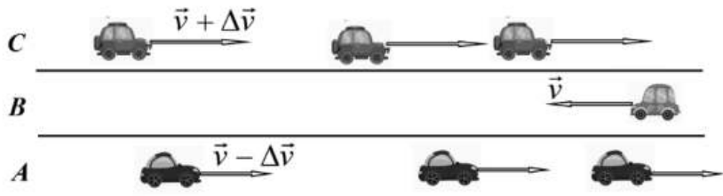
2.3 Calculate the number of cars $N_3$ in lane A and $N_4$ in lane C that the car B encounters within the time period of $t=1.0\text{min}$, as well as the corresponding times ${\tau }_3$ and ${\tau }_4$ between two consecutive encounters.

Elastic collision

In this part, we consider the classical problem of elastic collision of two bodies. The main purpose of this consideration is to determine the conditions under which the kinetic energy of one of the selected bodies increases as a result of the collision.

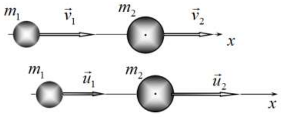
Two elastic balls, whose masses are equal to $m_1$ and $m_2$, respectively, move along the axis $x$. The speed of the first ball before the collision is $v_1$, whereas the speed of the second is $v_2$. Let us denote the speeds of the balls after an absolutely elastic central collision as $u_1$ and $u_2$, respectively. The speeds of the balls should be understood as the projections of their velocities on the $x$ axis, therefore, they can be both positive and/or negative.

2.4 Express the velocities of the balls $u_1$ and $u_2$ after the collision in terms of their velocities before the collision $v_1$ and $v_2$, as well as their masses.

Let us denote the ratio of the ball masses as $\mu =\frac{m_2}{m_1}$, the ratio of the speeds of the first ball after and before the collision as ${\eta }_1=\frac{u_1}{v_1}$ and the ratio of the velocities of the balls before the collision as ${\eta }_2=\frac{v_2}{v_1}$. For definiteness, consider that $v_1>0$.

2.5 Draw a set of graphs that represents the dependence of the parameter ${\eta }_1$ on the parameter ${\eta }_2$ for all characteristic values of the ball mass ratios $\mu$.

2.6 Find the relation between the parameters ${\eta }_2$ and $\mu$, at which the first ball increases its energy as a result of the collision.

2.7 Consider the case of a light ball colliding with a heavy one such that $m_2\gg m_1$. In this limiting case, find the speed of the first ball ${\tilde{u}}_1$ after the collision and determine the range of velocities ${\eta }_2$ of the heavy ball before the collision, at which the energy of the light ball increases as a result of the collision.

The simplest Fermi acceleration model

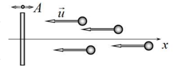
A massive plate, located perpendicular to the $x$ axis, performs harmonic oscillations in the direction of the $x$ axis. The oscillation amplitude is $A$ with the period being $T$. Light balls move with equal speeds $u$ in the direction of the plate along the $x$ axis such that the times of ball arrivals to the still plate are randomly and uniformly distributed.

2.8 Express the maximum speed of the plate $V_0$ in terms of the amplitude and period of its oscillations.

2.9 Calculate the fraction $\phi$ of incident balls that are to increase their kinetic energy after the collision. Express your answer in terms of $u$ and $V_0$. For a numerical estimate, consider the following two cases separately: a) $u=1.5V_0$; b) $u=0.50V_0$.

Let us approximate the harmonic law of the plate motion by a piecewise linear function, see the figure below, i.e. assume that the modulus of the plate speed remains constant at the same values of the amplitude and period of oscillations.

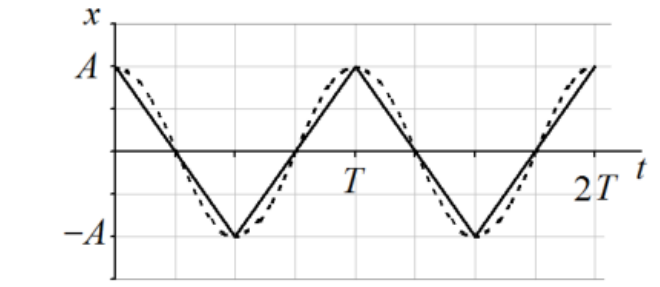
2.10 Express the value of the plate speed modulus $V$ in terms of the amplitude and period of its oscillations.

2.11 Calculate how many times $\epsilon =\frac{E}{E_0}$ the average energy of the incident balls changes, where $E_0$ is the kinetic energy of the balls before the collision, and $E$ symbolizes the average energy of the balls after the collision with the oscillating plate. For a numerical estimate, consider the following two cases separately: a) $u=1.5V$; b) $u=0.50V$.

Topic: Newtonian Mechanics Metodi: Conservation of Momentum, Energy Conservation Method Competenze: Mathematical Modeling, Physical Reasoning

Problema 2. Accelerazione di Fermi (10,0 punti)

I raggi cosmici contengono particelle ad energia estremamente elevata. Un possibile meccanismo per la formazione di tali particelle è chiamato accelerazione di Fermi.

L’accelerazione di Fermi è un processo stocastico attraverso il quale le particelle cariche subiscono un aumento di velocità quando vengono ripetutamente riflesse, solitamente da specchi magnetici. In questo problema esamineremo le principali idee alla base di questo fenomeno, a prima vista paradossale.

Perché le auto che vengono incontro sono più di quelle che sorpassano?

Su un’autostrada con tre corsie A, B, C, le automobili si muovono a velocità costante nella stessa direzione: lungo la corsia centrale B, un’automobile viaggia a una velocità di $v=90\text{km/h}$; le automobili sulla corsia A viaggiano a velocità $v-\Delta v=80\text{km/h}$; quelle sulla corsia C viaggiano a velocità $v+\Delta v=100\text{km/h}$. La distanza tra le automobili è la stessa su entrambe le corsie A e C, e il numero di automobili per unità di lunghezza di corsia è $n=5,0{\text{km}}^{-1}$ in entrambi i casi.

Si consideri l’auto che si muove nella corsia B.

2.1 Calcolare quante auto $N_1$ presenti nella corsia A sorpassino l’auto B nell’arco di tempo di $t=1,0\text{min}$, nonché il tempo ${\tau }_1$ che intercorre tra due sorpassi consecutivi.

2.2 Calcolare quante auto $N_2$ presenti nella corsia C sorpassino l’auto nella corsia B nell’arco di tempo di $t=1,0\text{min}$, nonché il tempo ${\tau }_2$ che intercorre tra due sorpassi consecutivi.

Ora si supponga che l’auto nella corsia B si muova verso le auto presenti nelle corsie A e C. Le velocità di tutte le auto, nonché la loro densità in ciascuna corsia, rimangono invariate.

2.3 Calcolare il numero di automobili $N_3$ nella corsia A e $N_4$ nella corsia C che l’automobile B incontra nel periodo di tempo $t=1,0\text{min}$, nonché i tempi corrispondenti ${\tau }_3$ e ${\tau }_4$ tra due incontri consecutivi.

Urto elastico

In questa parte consideriamo il problema classico dell’urto elastico tra due corpi. Lo scopo principale di questo studio è determinare le condizioni sotto cui l’energia cinetica di uno dei corpi aumenta a seguito della collisione.

Due palline elastiche, la cui massa è rispettivamente $m_1$ e $m_2$, si muovono lungo l’asse $x$. La velocità della prima pallina prima dell’impatto è $v_1$, mentre quella della seconda è $v_2$. Indichiamo con $u_1$ e $u_2$ le velocità delle palline dopo un impatto centrale completamente elastico. Le velocità delle palline vanno intese come le proiezioni delle loro velocità sull’asse $x$, pertanto possono essere sia positive che negative.

2.4 Esprimere le velocità $u_1$ e $u_2$ delle palline dopo l’impatto in termini delle velocità $v_1$ e $v_2$ prima dell’impatto, nonché delle loro masse.

Indichiamo con $\mu =\frac{m_2}{m_1}$ il rapporto tra le masse delle due palline, con ${\eta }_1=\frac{u_1}{v_1}$ il rapporto tra la velocità della prima pallina dopo e prima dell’impatto, e con ${\eta }_2=\frac{v_2}{v_1}$ il rapporto tra le velocità delle due palline prima dell’impatto. Per semplicità, si assuma che $v_1>0$.

2.5 Disegnare un insieme di grafici che rappresentino la dipendenza del parametro ${\eta }_1$ dal parametro ${\eta }_2$ per tutti i valori caratteristici del rapporto tra le masse delle palline, $\mu$.

2.6 Trovare la relazione tra i parametri ${\eta }_2$ e $\mu$ per cui la prima pallina aumenta la propria energia a seguito dell’impatto.

2.7 Si consideri il caso in cui una pallina leggera collide con una pesante, tale che $m_2\gg m_1$. In questa situazione limite, determinare la velocità della prima pallina ${\tilde{u}}_1$ dopo la collisione e individuare l’intervallo di velocità ${\eta }_2$ della pallina pesante prima dell’impatto, entro il quale l’energia della pallina leggera aumenta a seguito della collisione.

Il modello più semplice di accelerazione di Fermi

Una lastra massiccia, posizionata perpendicolarmente all’asse $x$, esegue oscillazioni armoniche nella direzione di questo asse. L’ampiezza delle oscillazioni è $A$ e il periodo è $T$. Palline leggere si muovono con uguali velocità $u$ verso la lastra lungo l’asse $x$, in modo che i tempi di arrivo delle palline alla lastra ferma siano distribuiti in modo casuale e uniforme.

2.8 Esprimere la velocità massima della lastra, $V_0$, in termini di ampiezza e periodo delle sue oscillazioni.

2.9 Calcolare la frazione $\phi$ di palline incidenti che aumentano la propria energia cinetica dopo la collisione. Esprimere la risposta in termini di $u$ e $V_0$. Per una stima numerica, considerare separatamente i seguenti due casi: a) $u=1,5V_0$; b) $u=0,50V_0$.

Approssimiamo la legge armonica del movimento della lastra con una funzione lineare a tratti, come mostrato nella figura sottostante; in altre parole, assumiamo che il modulo della velocità della lastra rimanga costante per gli stessi valori di ampiezza e periodo delle oscillazioni.

2.10 Esprimere il valore del modulo della velocità della lastra, $V$, in termini di ampiezza e periodo delle sue oscillazioni.

2.11 Calcolare quante volte $\epsilon =\frac{E}{E_0}$ cambia l’energia media delle palline incidenti, dove $E_0$ è l’energia cinetica delle palline prima della collisione e $E$ rappresenta l’energia media delle palline dopo la collisione con la lastra oscillante. Per una stima numerica, considerare separatamente i seguenti due casi: a) $u=1,5V$; b) $u=0,50V$.

Problem 3. Magnetron (10.0 points)

Both electric and magnetic fields act on moving charged particles, which in a certain way change the character of their motion. Everywhere below it is assumed that charged particles move in a vacuum, and the radiation of electromagnetic waves can be neglected.

In this problem, the motion of electrons, which are classical point-like particles, is considered. When carrying out numerical calculations, consider, where necessary, that an electron has a negative electric charge, whose modulus is equal to $e=1.60\cdot 10^{-19}\text{Cl}$, and its mass is $m=9.11\cdot 10^{-31}\text{kg}$. The electric and magnetic constants are equal ${\epsilon }_0=8.85\cdot 10^{-12}\text{F/m}$ and ${\mu }_0=1.26\cdot 10^{-6}\text{H/m}$, respectively, the Boltzmann constant is denoted as $k_B=1.38\cdot 10^{-23}\text{J/K}$.

Electron motion in electric and magnetic fields

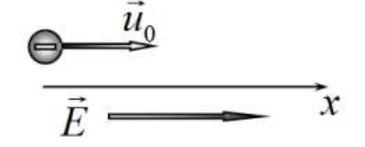
At the initial moment of time $t=0$ an electron is at rest at the origin of coordinates, and a uniform electric field with the strength $E$ is applied along the positive direction of the $x$ axis. The electron is given an initial velocity $u_0$, also directed in the positive direction of the $x$ axis.

3.1 Determine the maximum value of the electron coordinate $x_{max}$ for the entire time of its motion.

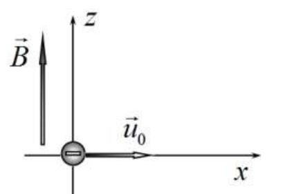
Now, at the initial moment of time $t=0$, an electron is at rest at the origin of coordinates, and a uniform magnetic field with the induction $B$ is applied along the positive direction of the $z$ axis. The electron is given an initial velocity $u_0$ directed in the positive direction of the $x$ axis.

3.2 Determine the maximum value of the electron coordinate $x_{max}$ for the entire time of its motion.

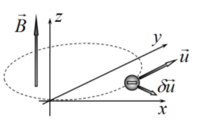
3.3 In the process of moving along the trajectory, at some moment of time, an additional velocity $\delta u$ is given to the electron in the direction perpendicular to its current velocity $u$ and lying in the plane of its initial trajectory, such that $\delta u\ll u$. Determine the period of the arisen two-dimensional oscillations of the electron with respect to its initial unperturbed trajectory.

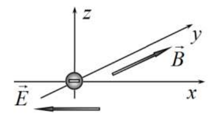
Again, at the initial moment of time $t=0$ an electron is at rest at the origin of coordinates, and a uniform electric field with the strength $E$ is applied along the negative direction of the $x$ axis. In addition, a uniform magnetic field with induction $B$ is created along the positive direction of the $y$ axis. The electron is released with the zero initial velocity.

3.4 Determine the maximum value of the electron coordinate $x_{max}$ for the entire time of its motion.

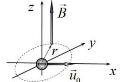
At the initial moment of time $t=0$ an electron is at rest at the origin of coordinates, and a magnetic field is applied along the positive direction of the $z$ axis, such that the induction in the plane $xy$ depends on the distance $r$ to the $z$ axis according to the law $B=\alpha r=\alpha (x^2+y^2{)}^{1/2}$. The electron is given an initial velocity directed in the positive direction of the $x$ axis.

3.5 Determine the maximum distance $r_{max}$ from the electron to the $z$ axis for the entire time of its motion.

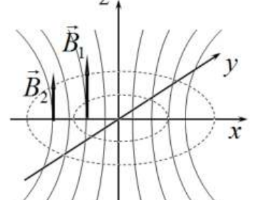
In some region of space, an axisymmetric magnetic field is created with respect to the $z$ axis. At the moment of time $t=0$, the magnetic field is absent, and then it begins to slowly increase, such that at all points in the $xy$ plane the field induction vector is directed along the $z$ axis. After a certain period of time, the induction of the magnetic field reaches its final value and ceases to change. The final field distribution in the $xy$ plane has the form

$B(r)=\{\begin{array}{ll}{B}_1,& 0<r\le r_1\\ B_2,& r_1<r\le r_2,\\ 0,& r>r_2\end{array}$

where $r$ denotes the distance to the $z$ axis, $r_1$ and $r_2$ are known quantities.

At a moment in time $t=0$, the electron is at rest at some point lying in the $xy$ plane. When the field is turned on, the electron begins to move along a circle in the $xy$ plane, whose center lies on the $z$ axis.

3.6 Determine under what conditions for the ratio $B_1/B_2$ the described situation turns possible.

Cylindrical magnetron

Magnetron is an electronic electrovacuum device, in which the amount of flowing current is controlled by electric and magnetic fields. Let us consider the simplest magnetron, consisting of a conducting coaxial long cylindrical cathode and anode with radii $a=3.00\cdot 10^{-1}\text{mm}$ and $b=6.00\text{mm}$, respectively, located inside a vacuum tube. The lamp is placed in the center of a cylindrical solenoid, whose axis coincides with the axes of the cathode and anode, and the number of turns is $N=2590$ with the length being equal $L=210\text{mm}$ and the diameter of $D=105\text{mm}$. The potential difference between the cathode and the anode is constant and equal to $V_0=75.0\text{V}$. Consider that the electrons leaving the cathode are formed due to thermionic emission and have a zero initial velocity, neglect the space charge of the electron cloud in the lamp.

3.7 Calculate the potential difference $V$ between the cathode and a point in space located at a distance $r=3.00$ мм from the common axis of the solenoid and the lamp.

3.8 Calculate the smallest solenoid current $I_{min}$ at which the current in the magnetron between the cathode and anode vanishes completely.

3.9 Find the condition for the cathode temperature $T$, under which the initial electron velocity can indeed be considered zero.

Mathematical hints for the theoretical problems. The following formulas may be useful: $\int x^{n}dx=\frac{x^{n+1}}{n+1}+C,\text{where }n\ne -1\text{ is a fixed number, }C\text{ refers to an arbitrary constant;}$ $\int \frac{dx}{x}=\ln |x|+C,\text{where }C\text{ stands for an arbitrary constant;}$ $\int \frac{dx}{(x^2+a^2{)}^{3/2}}=\frac{x}{a^2(x^2+a^2{)}^{1/2}}+C,\text{where }a,C\text{ stand for arbitrary constants;}$ $(1+x{)}^{\gamma }\approx 1+\gamma x+\frac{\gamma (\gamma -1)}{2}{x}^2,\text{for }|x|\ll 1\text{ and arbitrary }\gamma ;$ $\ln (1+x)\approx x,\text{for }|x|\ll 1.$

Topic: Magnetism, Electrostatics Metodi: Lorentz Force Analysis, Electric Potential Method Competenze: Mathematical Modeling, Physical Reasoning

Problema 3. Magnetron (10,0 punti)

Sia i campi elettrici che quelli magnetici agiscono sulle particelle cariche in movimento, modificandone in qualche modo il comportamento. In tutto il problema si assume che le particelle cariche si muovano nel vuoto e che la radiazione delle onde elettromagnetiche possa essere trascurata.

In questo caso viene considerato il movimento degli elettroni, che sono particelle puntiformi classiche. Nella realizzazione dei calcoli numerici, si tenga presente che un elettrone presenta una carica elettrica negativa il cui modulo è pari a $e=1,60\cdot 10^{-19}\text{Cl}$, e che la sua massa è di $m=9,11\cdot 10^{-31}\text{kg}$. Le costanti elettrica e magnetica sono rispettivamente ${\epsilon }_0=8,85\cdot 10^{-12}\text{F/m}$ e ${\mu }_0=1,26\cdot 10^{-6}\text{H/m}$, mentre la costante di Boltzmann è indicata con $k_B=1,38\cdot 10^{-23}\text{J/K}$.

Movimento dell’elettrone nei campi elettrico e magnetico

Nel momento iniziale $t=0$, un elettrone si trova a riposo nell’origine delle coordinate, mentre un campo elettrico uniforme di intensità $E$ viene applicato lungo la direzione positiva dell’asse $x$. All’elettrone viene inoltre data una velocità iniziale $u_0$, anch’essa diretta nella stessa direzione.

3.1 Determinare il valore massimo $x_{max}$ della coordinata dell’elettrone nel corso di tutto il suo moto.

Nel momento iniziale, quando $t=0$, un elettrone si trova a riposo nell’origine delle coordinate, mentre un campo magnetico uniforme con induzione $B$ viene applicato lungo la direzione positiva dell’asse $z$. All’elettrone viene data una velocità iniziale $u_0$ diretta nella direzione positiva dell’asse $x$.

3.2 Determinare il valore massimo della coordinata $x$ dell’elettrone, $x_{max}$, per l’intero arco del suo movimento.

3.3 Nel corso del suo movimento lungo la traiettoria, in un certo istante di tempo, all’elettrone viene impartita una velocità aggiuntiva $\delta u$ nella direzione perpendicolare alla sua velocità attuale $u$, e tale velocità aggiuntiva si trova nel piano della sua traiettoria iniziale; si suppone che $\delta u\ll u$. Determinare il periodo delle oscillazioni bidimensionali che ne derivano, rispetto alla sua traiettoria iniziale non perturbata.

Ancora una volta, al momento iniziale $t=0$, un elettrone si trova a riposo nell’origine delle coordinate; inoltre, viene applicato un campo elettrico uniforme di intensità $E$ lungo la direzione negativa dell’asse $x$. Allo stesso tempo, viene generato un campo magnetico uniforme di induzione $B$ lungo la direzione positiva dell’asse $y$. L’elettrone viene rilasciato con velocità iniziale nulla.

3.4 Determinare il valore massimo della coordinata $x$ dell’elettrone, $x_{max}$, per l’intero arco del suo movimento.

Nel momento iniziale $t=0$, un elettrone si trova a riposo nell’origine delle coordinate, mentre un campo magnetico viene applicato lungo la direzione positiva dell’asse $z$, tale che l’induzione $B$ nel piano $xy$ dipenda dalla distanza $r$ dall’asse $z$ secondo la legge $B=\alpha r=\alpha (x^2+y^2{)}^{1/2}$. All’elettrone viene inoltre data una velocità iniziale diretta nella direzione positiva dell’asse $x$.

3.5 Determinare la massima distanza $r_{max}$ che l’elettrone può raggiungere rispetto all’asse $z$ durante tutto il corso del suo movimento.

In una certa regione dello spazio viene creato un campo magnetico assialmente simmetrico rispetto all’asse $z$. Nel momento $t=0$ il campo magnetico è assente, per poi iniziare ad aumentare lentamente, in modo che in tutti i punti del piano $xy$ il vettore di induzione del campo sia diretto lungo l’asse $z$. Dopo un certo periodo di tempo, l’induzione del campo magnetico raggiunge il suo valore finale e smette di variare. La distribuzione finale del campo nel piano $xy$ ha la seguente forma:

$B(r)=\{\begin{array}{ll}{B}_1,& 0<r\le r_1\\ B_2,& r_1<r\le r_2,\\ 0,& r>r_2\end{array}$

dove $r$ indica la distanza dall’asse $z$, $r_1$ e $r_2$ sono quantità note.

In un istante di tempo $t=0$, l’elettrone si trova a riposo in un punto situato nel piano $xy$. Quando il campo viene attivato, l’elettrone inizia a muoversi lungo un cerchio nel piano $xy$, il cui centro si trova sull’asse $z$.

3.6 Determinare sotto quali condizioni, per il rapporto $B_1/B_2$, la situazione descritta diventa possibile.

Magnetron cilindrico

Il magnetron è un dispositivo elettronico a vuoto in cui la quantità di corrente che scorre viene controllata da campi elettrici e magnetici. Consideriamo il magnetron più semplice, costituito da un catodo e un anodo cilindrici conduttori e coassiali, con raggi rispettivamente $a=3,00\cdot 10^{-1}\text{mm}$ e $b=6,00\text{mm}$, posizionati all’interno di un tubo a vuoto. Il tubo è posto al centro di un solenoide cilindrico, il cui asse coincide con gli assi del catodo e dell’anodo; il numero di spire è $N=2590$, la lunghezza è $L=210\text{mm}$ e il diametro è $D=105\text{mm}$. La differenza di potenziale tra catodo e anodo è costante e uguale a $V_0=75,0\text{V}$. Si consideri che gli elettroni che lasciano il catodo si formano per emissione termionica e hanno una velocità iniziale zero; si trascuri inoltre la carica spaziale della nube di elettroni all’interno del tubo.

3.7 Calcolare la differenza di potenziale $V$ tra il catodo e un punto dello spazio situato a una distanza $r=3,00$ мм dall’asse comune del solenoide e del tubo.

3.8 Calcolare la minima corrente nel solenoide $I_{min}$ tale che la corrente nel magnetron, tra catodo e anodo, scompaia completamente.

3.9 Determinare la condizione relativa alla temperatura del catodo $T$ per cui la velocità iniziale degli elettroni possa effettivamente essere considerata zero.

Suggerimenti matematici per i problemi teorici. Le seguenti formule possono rivelarsi utili: $\int x^{n}dx=\frac{x^{n+1}}{n+1}+C,\text{dove }n\ne -1\text{ eˋ un numero fisso, }C\text{ rappresenta una costante arbitraria;}$ $\int \frac{dx}{x}=\ln |x|+C,\text{dove }C\text{ indica una costante arbitraria;}$ $\int \frac{dx}{(x^2+a^2{)}^{3/2}}=\frac{x}{a^2(x^2+a^2{)}^{1/2}}+C,\text{dove }a,C\text{ sono costanti arbitrarie;}$ $(1+x{)}^{\gamma }\approx 1+\gamma x+\frac{\gamma (\gamma -1)}{2}{x}^2,\text{per }|x|\ll 1\text{ e qualsiasi valore di }\gamma ;$ $\ln (1+x)\approx x,\text{per }|x|\ll 1.$