IZhO 2026

Problem 1 (10.0 points)

Theoretical competition — January 11, 2026 (XXII IZhO).

This problem consists of three independent parts.

Problem 1.1 (3.0 points)

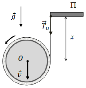
A thin cylindrical core of radius $R$ has a strip of foil tightly wound around it in a thin layer. The foil has thickness $\delta$, mass $m$, and length $L=10.0$ m. One end of the foil is fixed to the core, while the other end is attached to the edge of a thin horizontal platform $\Pi$. Initially, the roll (the core with the wound foil) is held so that its axis $O$ is horizontal and at the same level as the platform. The roll is then released, and under the action of gravity it begins to unwind. Assuming that $\delta \ll R\ll L$, find the length $x_0$ of the unwound part of the foil for which the force $T_0$ acting on the platform is equal to the weight of the roll, $mg$. Also determine the acceleration $a$ and the velocity $v$ of the downward motion of the roll’s center of mass at that instant.

Problem 1.2 (4.0 points)

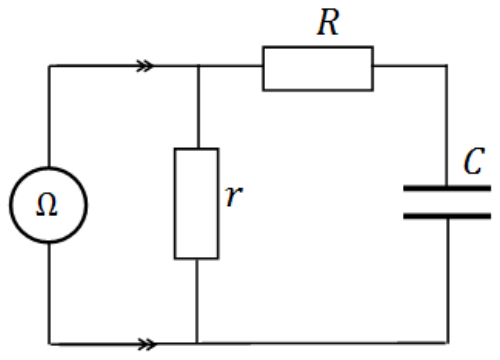
The readings of a multimeter ($\Omega$) operating in ohmmeter mode and connected to a circuit change with time according to the law $R_{\Omega }(t)=A-B{e}^{-t/{\tau }_0}$, where $A=100$ kΩ, $B=40$ kΩ, and ${\tau }_0=100$ s. Using these data, determine the values of the resistances $r$ and $R$, as well as the capacitance $C$ of the capacitor, which is initially uncharged. Also find the amount of heat $Q$ released in the resistor $R$ during the measurement time $t\gg {\tau }_0$.

Note: In ohmmeter mode, the multimeter measures the voltage drop $U_x$ across an unknown resistor $R_x$ when a constant current $I_0=0.1$ mA flows through it. The instrument displays the value $R_x=U_x/I_0$.

Problem 1.3 (3.0 points)

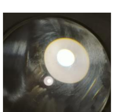
An observer (the eye) is located at a distance $L=55$ cm from a convex–concave lens and observes images of a distant street lamp formed due to reflections from both surfaces of the lens (see photo). The lamp and the eye are positioned close to the principal optical axis of the lens on the side of the concave surface. The radius of curvature of the concave surface is $r=7$ cm, and the radius of curvature of the convex surface is $R=28$ cm. Upon observation, two images of the lamp are visible: one real and the other virtual. The ratio of the apparent angular sizes of these images is $\gamma ={\phi }_1/{\phi }_2=0.1$, where ${\phi }_1$ is the angular size of the real image and ${\phi }_2$ is the angular size of the virtual image. Find the optical power $D$ of the lens.

Topic: Rotational Dynamics, Circuits, Geometric Optics Metodi: Energy Conservation Method, Differential Equations, Thin Lens & Mirror Equation Competenze: Mathematical Modeling, Physical Reasoning

Problema 1 (10,0 punti)

Prova teorica — 11 gennaio 2026 (XXII IZhO).

Questo problema è composto da tre parti indipendenti.

Problema 1.1 (3,0 punti)

Un sottile nucleo cilindrico di raggio $R$ presenta una striscia di lamina sottile avvolta strettamente attorno ad esso in uno strato sottile. La lamina ha uno spessore $\delta$, una massa $m$ e una lunghezza $L=10,0$ m. Un’estremità della lamina è fissata al nucleo, mentre l’altra estremità è collegata al bordo di una sottile piattaforma orizzontale $\Pi$. Inizialmente, il rotolo (il nucleo con la lamina avvolta) viene tenuto in modo che il suo asse $O$ sia orizzontale e allo stesso livello della piattaforma. Successivamente, il rotolo viene rilasciato e, sotto l’azione della gravità, inizia a srotolarsi. Supponendo che $\delta \ll R\ll L$, determinare la lunghezza $x_0$ della parte di lamina già srotolata per cui la forza $T_0$ agente sulla piattaforma è uguale al peso del rotolo, $mg$. Determinare inoltre l’accelerazione $a$ e la velocità $v$ del moto verso il basso del centro di massa del rotolo in quell’istante.

Problema 1.2 (4,0 punti)

Le letture di un multimetro ($\Omega$) funzionante in modalità ohmmetro e collegato a un circuito variano nel tempo secondo la legge $R_{\Omega }(t)=A-B{e}^{-t/{\tau }_0}$, dove $A=100$ kΩ, $B=40$ kΩ e ${\tau }_0=100$ s. Utilizzando questi dati, determinare i valori delle resistenze $r$ e $R$, nonché la capacità $C$ del condensatore, che inizialmente è scarico. Calcolare inoltre la quantità di calore $Q$ rilasciata nella resistenza $R$ durante il tempo di misurazione $t\gg {\tau }_0$.

Nota: In modalità ohmmetro, il multimetro misura la caduta di tensione $U_x$ attraverso una resistenza sconosciuta $R_x$ quando attraverso di essa scorre una corrente costante $I_0=0,1$ mA. Lo strumento visualizza il valore $R_x=U_x/I_0$.

Problema 1.3 (3,0 punti)

Un osservatore (l’occhio) si trova a una distanza di $L=55$ cm da una lente convessa-concava e osserva le immagini di un lampione lontano, formatesi a seguito delle riflessioni su entrambe le superfici della lente (vedi foto). Il lampione e l’occhio sono posizionati vicino all’asse ottico principale della lente, sul lato della superficie concava. Il raggio di curvatura della superficie concava è $r=7$ cm, mentre il raggio di curvatura della superficie convessa è $R=28$ cm. Durante l’osservazione, sono visibili due immagini del lampione: una reale e l’altra virtuale. Il rapporto delle dimensioni angolari apparenti di queste immagini è $\gamma ={\phi }_1/{\phi }_2=0,1$, dove ${\phi }_1$ rappresenta la dimensione angolare dell’immagine reale e ${\phi }_2$ quella dell’immagine virtuale. Determinare la potenza ottica $D$ della lente.

Problem 2. Steam Engine (10.0 points)

In this problem, we consider a simplified theoretical model of one type of steam engine. Note that at present such an engine is used only as a technical toy.

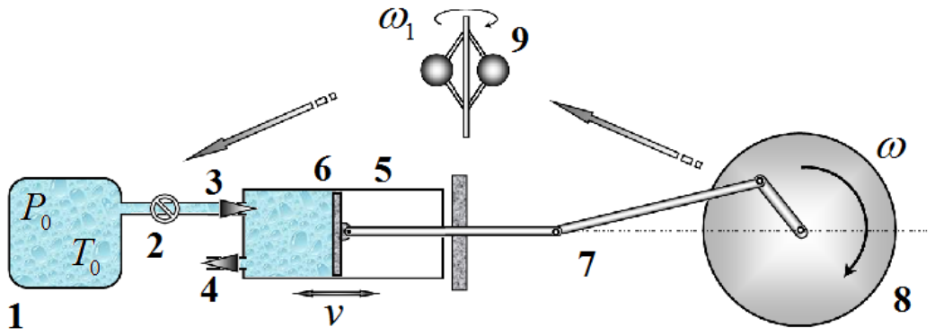
A schematic diagram of the engine under consideration is shown in the figure above. There is a steam generator 1 (a boiler with water and a heater, as well as a system for additional superheating of the steam). The generator may be regarded as a large vessel containing water vapor (without air), in which the pressure $P_0$ and temperature $T_0$ are maintained constant. The heated steam is supplied through a pipe to the working cylinder 5 with a movable piston 6. The pipe is equipped with a steam supply regulator 2 controlled by a Watt centrifugal governor 9. The working cylinder has two valves: an inlet valve 3 and an outlet valve 4. These valves open and close at certain positions of the piston. The movable piston is connected to a system of rods 7 that converts the translational motion of the piston into rotational motion of a massive flywheel 8 mounted on the engine shaft. By means of a belt drive, this wheel is connected to the Watt governor, whose angular velocity $\omega$ is equal to the angular velocity of the flywheel. The amount of steam passing through the steam supply regulator 2 depends on the rotational frequency of the governor. The flywheel shaft is connected to the working device (for whose sake all engines are created).

In all parts of the problem, steady operating regimes are considered, in which the angular velocities of rotation of the shaft and the Watt governor remain constant. Of course, the transition to such regimes is possible only in the presence of friction; however, in calculations of the steady motion, friction may be neglected.

Assume that the adiabatic index of water is $\gamma =4/3$, the molar mass of water is $M=18.0\cdot 10^{-3}$ kg/mole.

Part 1. Steam Engine without a Governor

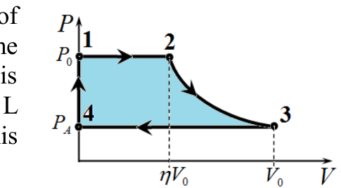
The ideal cycle of the engine under consideration in the limit of infinitely slow motion is shown on the $P-V$ diagram. Here $V$ is the volume of the part of the cylinder between the cylinder end face and the piston that is occupied by steam (hereafter referred to as the working volume); $V_0=4.00$ L is the maximum working volume; and $P$ is the pressure of the steam in this volume.

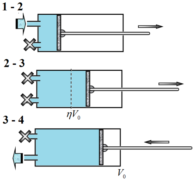
In state 1, the piston touches the cylinder wall and the working volume is zero. The inlet valve opens, and steam begins to enter the cylinder. Along segment 1 – 2 of the cycle, the piston moves slowly to the right; in this process, the steam pressure in the cylinder may be assumed to be equal at all times to the pressure of the steam in the generator, $P_0=10.0\cdot 10^5$ Pa.

At point 2, when the working volume reaches the value $\eta V_0$, the inlet valve closes, and the piston continues to move to the right under the action of the steam pressure. Along segment 2 – 3, the expansion process is adiabatic.

At point 3, the piston reaches its extreme position, the working volume is maximal, and the pressure drops to the atmospheric value $P_A=1.00\cdot 10^5$ Pa. After that, the outlet valve opens, and the piston expels the steam into the atmosphere.

When the piston returns to the extreme left position, the outlet valve closes and the inlet valve opens again (segment 4 – 1).

2.1 Determine the value of the coefficient $\eta$.

To prevent steam condensation, its minimum temperature must be higher than the condensation temperature at atmospheric pressure, $t_S=100$ °C.

2.2 Determine the required value of the steam temperature $T_0$ (in degrees Celsius) such that during the expansion process the temperature does not drop below the condensation temperature $t_S$.

In what follows, assume that in the considered model the parameters $T_0$ and $\eta$ are equal to the values found above.

2.3 Calculate the mass of steam $m_0$ entering the cylinder during one cycle.

2.4 Calculate the work $A_0$ performed by the engine during one cycle.

Next, consider the operation of the engine in a real regime, taking into account that the piston moves with some finite velocity. Assume that the flywheel rotates with a constant angular velocity $\omega$. Strictly speaking, in this case the motion of the piston is not uniform. However, as an approximation, the piston velocity in one direction may be taken to be constant and equal to its average velocity. In this problem, it is convenient to consider the rate of change of the working volume, $v=dV/dt$.

2.5 Express the average rate of change of the working volume of the cylinder $v$ in terms of the maximum working volume $V_0$ and the angular velocity $\omega$ of the flywheel.

During the piston motion, the steam pressure $P$ in the cylinder during stage 1 – 2 of the cycle differs from the steam pressure in the generator $P_0$. Assume that the rate of steam inflow is proportional to the pressure difference across the steam regulator 2, i.e.,

$\frac{dm}{dt}=K(P_0-P),$

where $K$ is a constant coefficient determined by regulator 2. In this part, take it to be constant and equal to $K=K_0=4.20\cdot 10^{-7}$ kg/(Pa·s).

Assume that the steam expansion process at all stages of the cycle is adiabatic.

2.6 Derive a differential equation describing the change in the mass of gas in the cylinder while the inlet valve is open. Besides the unknown function $m(t)$, this equation should contain only known quantities.

2.7 Show that at a constant piston velocity the steam pressure $P$ in the cylinder remains constant.

2.8 Obtain an algebraic equation for determining the steam pressure $P$ in the cylinder during stage 1 – 2 of the cycle.

To approximately solve the resulting equation (i.e., to find the pressure $P$), make the following mathematical approximation: assume (only in this part of the problem) that the adiabatic index of water vapor is $\gamma \approx 1$. In addition, when calculating the work performed by the steam, neglect atmospheric pressure.

2.9 Using the above approximation, express the steam pressure $P$ in the cylinder during stage 1 – 2 in terms of the pressure $P_0$ and the other known parameters of the problem.

2.10 Calculate the numerical value of the pressure $P$ at an angular velocity of the shaft $\omega =10.0$ s⁻¹.

2.11 Show that the formula for calculating the work $A$ performed by the engine during one cycle when the flywheel rotates with a constant angular velocity $\omega$ can be written in the form $A=\frac{A_0}{1+\beta /K}$. Calculate the numerical values of the parameters $A_0$ and $\beta$ in this formula.

Assume that, in addition to the torque $M$ exerted by the piston, a constant torque $M_0$ from the working device acts on the engine shaft.

2.12 Express the average steady-state angular velocity $\omega$ of the wheel in terms of the torque $M_0$, the coefficient $K$, and the parameters $A_0$ and $\beta$.

2.13 Calculate the maximum torque $M_0$ at which the engine can operate.

2.14 Sketch a schematic graph of the dependence of the angular velocity of rotation on the torque $M_0$.

Part 2. Governor without the Engine

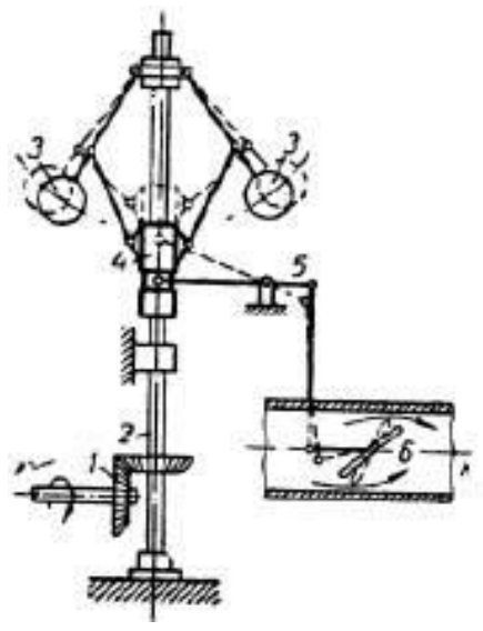
The angular velocity of rotation of the engine flywheel depends on the torque transmitted to the working device. When this torque decreases, the angular velocity may increase sharply, which can lead to engine failure and its further destruction. To avoid such situations, various automatic control systems are used, one of which is the Watt centrifugal governor.

The principle of its operation is quite simple. The rotation of the engine shaft is transmitted through a drive to the shaft of the governor. During the rotation of the governor shaft, the balls deviate from the axis under the action of the centrifugal force; the faster the shaft rotates, the farther apart the balls move. The levers interact with a sleeve and move it along the shaft axis. Through a system of levers, the displacement of the sleeve is transmitted to the steam supply throttle in such a way that when the rotational speed of the shaft increases, the steam supply decreases, and when it decreases, the steam supply increases.

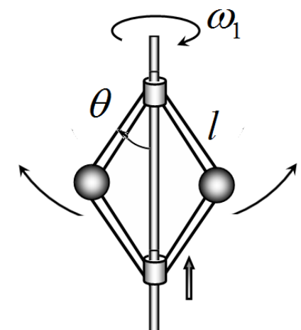
For solving this problem, the technical details of the specific device are not essential. Let us consider an idealized schematic model of the governor. A hinged rhombic frame is mounted on a vertical shaft rotating with a constant angular velocity $\omega$. The upper vertex of the frame is fixed, while the lower vertex can freely slide along the shaft. Two massive balls are attached at the lateral vertices of the frame. It may be assumed that in the absence of shaft rotation $\theta =0$. When the shaft rotates, the balls rise, deviating by an angle $\theta$ from the vertical. This leads to a reduction in the steam supply to the working cylinder. We assume that the coefficient $K$, which characterizes the steam flow rate, is related to the deflection angle by the simple relation

$K=K_0\cos \theta ,$

where $K_0$ is the coefficient defined earlier.

The length of a side of the frame is $l=20$ cm.

2.15 Find the dependence of the deflection angle $\theta$ of the balls from the vertical on the constant angular velocity $\omega$ of the governor.

2.16 Sketch a schematic graph of the dependence of the coefficient $K$ on the angular velocity $\omega$ of the governor.

Part 3. Engine with a Governor

2.17 Find the dependence of the steady-state angular velocity of rotation of the engine shaft on the torque $M_0$ for the governor system described above.

2.18 Sketch a schematic graph of the resulting dependence.

Topic: Thermodynamics Metodi: Thermodynamic Cycle Analysis, First Law of Thermodynamics, Differential Equations Competenze: Mathematical Modeling, Physical Reasoning

Problema 2. Macchina a vapore (10,0 punti)

In questo problema consideriamo un modello teorico semplificato di un certo tipo di macchina a vapore. Si noti che attualmente tale macchina viene utilizzata soltanto come giocattolo tecnico.

Un diagramma schematico del motore in esame è mostrato nella figura sopra. È presente un generatore di vapore 1 (una caldaia contenente acqua e un riscaldatore, nonché un sistema per surriscaldare ulteriormente il vapore). Il generatore può essere considerato un grande recipiente che contiene vapore acqueo (senza aria), nel quale la pressione $P_0$ e la temperatura $T_0$ rimangono costanti. Il vapore riscaldato viene inviato attraverso un tubo al cilindro di lavoro 5, dotato di un pistone mobile 6. Il tubo è equipaggiato con un regolatore di alimentazione del vapore 2, controllato da un regolatore centrifugo di Watt 9. Il cilindro di lavoro presenta due valvole: una valvola di ingresso 3 e una valvola di uscita 4; queste valvole si aprono e si chiudono in corrispondenza di determinate posizioni del pistone. Il pistone mobile è collegato a un sistema di bielle 7 che converte il movimento traslatorio del pistone in movimento rotatorio di un volano massiccio 8 montato sull’albero del motore. Attraverso una trasmissione a cinghia, questo volano è collegato al regolatore di Watt, la cui velocità angolare $\omega$ è uguale a quella del volano stesso. La quantità di vapore che passa attraverso il regolatore 2 dipende dalla frequenza di rotazione del regolatore. L’albero del volano è collegato al dispositivo di lavoro (per il quale tutti i motori vengono costruiti).

In tutte le parti del problema vengono considerati regimi operativi stazionari, in cui la velocità angolare di rotazione dell’albero e del regolatore di Watt rimane costante. Naturalmente, il passaggio a tali regimi è possibile solo in presenza di attrito; tuttavia, nei calcoli relativi al movimento stazionario, l’attrito può essere trascurato.

Si assuma che l’indice adiabatico dell’acqua sia $\gamma =4/3$ e che la massa molare dell’acqua sia $M=18,0\cdot 10^{-3}$ kg/mole.

Parte 1. Macchina a vapore senza regolatore di velocità

Il ciclo ideale del motore in esame, nel limite di un movimento infinitamente lento, è rappresentato sul diagramma $P-V$. In questo contesto, $V$ indica il volume della parte del cilindro compresa tra la faccia terminale del cilindro e il pistone che è occupata dal vapore (da ora in poi denominato “volume di lavoro”); $V_0=4,00$ L rappresenta il volume di lavoro massimo; mentre $P$ indica la pressione del vapore all’interno di questo volume.

Nello stato 1, il pistone è a contatto con la parete del cilindro e il volume di lavoro è zero. La valvola di ingresso si apre e il vapore inizia ad entrare nel cilindro. Nel tratto 1–2 del ciclo, il pistone si muove lentamente verso destra; in questo processo, la pressione del vapore all’interno del cilindro può essere considerata costante e uguale alla pressione del vapore nel generatore, $P_0=10,0\cdot 10^5$ Pa.

Al punto 2, quando il volume di lavoro raggiunge il valore $\eta V_0$, la valvola di ingresso si chiude e il pistone continua a muoversi verso destra sotto l’azione della pressione del vapore. Nel tratto 2–3, il processo di espansione è adiabatico.

Al punto 3, il pistone raggiunge la sua posizione estrema, il volume di lavoro è massimo e la pressione scende al valore atmosferico $P_A=1,00\cdot 10^5$ Pa. Dopo di ciò, la valvola di uscita si apre e il pistone espelle il vapore nell’atmosfera.

Quando il pistone ritorna nella posizione estrema a sinistra, la valvola di uscita si chiude e la valvola di ingresso si apre nuovamente (tratto 4–1).

2.1 Determinare il valore del coefficiente $\eta$.

Per evitare la condensazione del vapore, la sua temperatura minima deve essere superiore alla temperatura di condensazione a pressione atmosferica, $t_S=100$ °C.

2.2 Determinare il valore necessario della temperatura del vapore $T_0$ (in gradi Celsius) in modo che durante il processo di espansione la temperatura non scenda al di sotto della temperatura di condensazione $t_S$.

Nel seguito, si assume che nel modello considerato i valori di $T_0$ e $\eta$ siano quelli determinati sopra.

2.3 Calcolare la massa di vapore $m_0$ che entra nel cilindro durante un ciclo completo.

2.4 Calcolare il lavoro $A_0$ eseguito dal motore durante un ciclo.

Si consideri poi il funzionamento del motore in regime reale, tenendo conto che il pistone si muove con una velocità finita. Si assuma che il volano giri a una velocità angolare costante $\omega$. In senso stretto, in questo caso il movimento del pistone non è uniforme. Tuttavia, come approssimazione, si può considerare la velocità del pistone in una direzione costante e uguale alla sua velocità media. In questo problema, è conveniente considerare la rapidità di variazione del volume di lavoro, $v=dV/dt$.

2.5 Esprimere la rapidità media di variazione del volume di lavoro del cilindro $v$ in termini del volume di lavoro massimo $V_0$ e della velocità angolare $\omega$ delil volano.

Durante il movimento del pistone, la pressione del vapore nel cilindro durante le fasi 1–2 del ciclo differisce dalla pressione del vapore nel generatore $P_0$. Si assuma che il flusso di vapore sia proporzionale alla differenza di pressione attraverso il regolatore di vapore 2, cioè

$\frac{dm}{dt}=K(P_0-P),$

dove $K$ è un coefficiente costante determinato dal regolatore 2; in questa parte, si assume che sia costante e uguale a $K=K_0=4,20\cdot 10^{-7}$ kg/(Pa·s).

Si assuma che il processo di espansione del vapore in tutte le fasi del ciclo sia adiabatico.

2.6 Derivare un’equazione differenziale che descriva la variazione della massa di gas nel cilindro quando la valvola di ingresso è aperta. Oltre alla funzione sconosciuta $m(t)$, questa equazione deve contenere soltanto quantità note.

2.7 Dimostrare che, a velocità costante del pistone, la pressione del vapore $P$ nel cilindro rimane costante.

2.8 Ottenere un’equazione algebrica per determinare la pressione del vapore $P$ nel cilindro durante la fase 1–2 del ciclo.

Per risolvere approssimativamente l’equazione risultante (cioè, per trovare la pressione $P$), si effettua la seguente approssimazione matematica: si assume (solo in questa parte del problema) che l’indice adiabatico del vapore acqueo sia $\gamma \approx 1$. Inoltre, nel calcolo del lavoro compiuto dal vapore, si ignora la pressione atmosferica.

2.9 Utilizzando la suddetta approssimazione, esprimere la pressione del vapore $P$ nel cilindro durante la fase 1–2 in termini di pressione $P_0$ e degli altri parametri noti del problema.

2.10 Calcolare il valore numerico della pressione $P$ a una velocità angolare dell’albero di $\omega =10,0$ s⁻¹.

2.11 Dimostrare che la formula per calcolare il lavoro $A$ eseguito dal motore durante un ciclo, quando il volano ruota con una velocità angolare costante $\omega$, può essere scritta nella forma $A=\frac{A_0}{1+\beta /K}$. Calcolare i valori numerici dei parametri $A_0$ e $\beta$ in questa formula.

Si assuma che, oltre al momento torcente $M$ esercitato dal pistone, un altro momento torcente costante $M_0$, proveniente dall’apparato di lavoro, agisca sull’albero del motore.

2.12 Esprimere la velocità angolare media in regime stazionario $\omega$ delil volano in termini di momento torcente $M_0$, coefficiente $K$ e parametri $A_0$ e $\beta$.

2.13 Calcolare il massimo momento torcente $M_0$ al quale il motore può funzionare.

2.14 Disegnare un grafico schematico che rappresenti la dipendenza della velocità angolare di rotazione dal momento torcente $M_0$.

Parte 2. Regolatore senza motore

La velocità angolare di rotazione del volano del motore dipende dal momento torcente trasmesso al dispositivo di lavoro. Quando questo momento torcente diminuisce, la velocità angolare può aumentare bruscamente, il che può portare al guasto del motore e alla sua ulteriore distruzione. Per evitare tali situazioni, vengono utilizzati vari sistemi di controllo automatico, tra cui il regolatore centrifugo di Watt.

Il principio del suo funzionamento è piuttosto semplice. La rotazione dell’albero del motore viene trasmessa, tramite un sistema di trasmissione, all’albero del regolatore. Durante la rotazione dell’albero del regolatore, le sfere si allontanano dall’asse sotto l’effetto della forza centrifuga; più veloce ruota l’albero, più le sfere si allontanano. Le leve presenti nel sistema interagiscono con un manicotto, spostandolo lungo l’asse dell’albero stesso. Attraverso questo meccanismo, lo spostamento del manicotto viene trasferito al regolatore del flusso di vapore: quando la velocità di rotazione aumenta, il flusso di vapore diminuisce; quando invece diminuisce, il flusso di vapore aumenta.

Per risolvere questo problema, i dettagli tecnici del dispositivo specifico non sono essenziali. Consideriamo un modello schematico idealizzato del regolatore. Un telaio rombico munito di articolazioni è montato su un albero verticale che ruota a una velocità angolare costante $\omega$. Il vertice superiore del telaio è fissata, mentre il vertice inferiore può scorrere liberamente lungo l’albero. Ai vertici laterali del telaio sono attaccate due sfere di massa considerevole. Si può assumere che, in assenza di rotazione dell’albero, l’angolo $\theta$ sia pari a 0. Quando l’albero ruota, le sfere si sollevano, deviando di un angolo $\theta$ rispetto alla verticale; ciò comporta una riduzione del flusso di vapore che raggiunge il cilindro di lavoro. Supponiamo che il coefficiente $K$, che caratterizza la portata di vapore, sia legato all’angolo di deviazione dalla semplice relazione

$K=K_0\cos \theta ,$

dove $K_0$ è il coefficiente definito in precedenza.

La lunghezza di un lato del telaio è $l=20$ cm.

2.15 Determinare in che modo l’angolo di deviazione $\theta$ delle sfere rispetto alla verticale dipenda dalla velocità angolare costante $\omega$ del regolatore.

2.16 Disegnare un grafico schematico che mostri la dipendenza del coefficiente $K$ dalla velocità angolare $\omega$ del regolatore.

Parte 3. Motore con regolatore

2.17 Determinare in che modo la velocità angolare di rotazione in regime stazionario dell’albero del motore dipenda dal momento torcente $M_0$ nel sistema di regolazione descritto sopra.

2.18 Disegnare un grafico schematico che mostri questa dipendenza.

Problem 3. Electron Paramagnetic Resonance (10.0 points)

Magnetic Moment

The magnetic moment $\mathbf{m}$ of a planar current loop is a vector quantity defined as the product of the electric current $I$, the area of the loop $S$, and the unit normal vector $\mathbf{n}$ perpendicular to the plane of the loop:

$\mathbf{m}=IS\mathbf{n}.$

The direction of the magnetic moment vector is determined by the right-hand (corkscrew) rule: if the fingers of the right hand curl in the direction of the current in the loop, the thumb points in the direction of $\mathbf{m}$.

3.1 A circular loop of radius $R$ carries an electric current and has a magnetic moment $\mathbf{m}$. Find the magnetic field induction ${\mathbf{B}}_0$ at the center of the loop.

3.2 The same loop is placed in an external uniform magnetic field of induction $\mathbf{B}$ such that the magnetic moment vector makes an angle $\phi$ with the direction of $\mathbf{B}$. Find the magnitude of the mechanical torque $M$ acting on the loop due to the external magnetic field.

3.3 The loop is slowly rotated in an external uniform magnetic field $\mathbf{B}$ so that the direction of its magnetic moment $\mathbf{m}$ changes from being aligned with the field ($\mathbf{m}\uparrow \mathbf{B}$) to being opposite to the field ($\mathbf{m}\downarrow \mathbf{B}$). Find the mechanical work $A$ done by the magnetic field during this rotation.

Electron Paramagnetic Resonance

If a charged particle rotates or moves along a closed trajectory, it possesses a mechanical (angular) momentum, and as a result a magnetic moment also arises. In this case, a universal gyromagnetic relation holds, which shows how the magnetic moment and the mechanical moment of the particle are related.

Suppose an electron in an atom moves along a circular orbit such that its orbital angular momentum with respect to the center is $\mathbf{L}$. Such motion can be regarded as equivalent to a circular electric current, which has a magnetic moment $\mathbf{m}$. The magnetic moment and the angular momentum are related by the gyromagnetic relation

$\mathbf{m}=-g_L\frac{e}{2m_e}\mathbf{L},$

where $e$ is the elementary charge, $m_e$ denotes the electron mass, and $g_L$ stands for the so-called Landé $g$-factor.

3.4 Find the Landé factor $g_L$ for the circular orbital motion of an electron.

Electron Paramagnetic Resonance (EPR) is a phenomenon in which a substance containing unpaired electrons absorbs electromagnetic radiation (usually in the microwave range) when placed in a constant magnetic field. This absorption does not occur at arbitrary frequencies but only at a strictly defined one, and is therefore called resonant.

Assume that an atom has a single unpaired electron in its outer shell with zero orbital angular momentum. Such an electron has an intrinsic angular momentum called spin. When a sample of the substance is placed in a constant magnetic field produced by a solenoid with magnetic induction $B$, the spin can be oriented in two ways relative to the field: along the magnetic field direction with angular momentum projection $+\hslash /2$, or opposite to it with projection $-\hslash /2$. These two orientations have different energies, so transitions between them are possible. In what follows, assume that the Landé factor for the spin, $g_s$, is twice that for the electron’s orbital motion. The sample is irradiated with an electromagnetic wave of fixed angular frequency $\omega$, which can induce transitions of the electron between the two states with different spin projections. Then the magnitude of the external magnetic field induction is slowly varied, while the change in the absorption intensity of the electromagnetic radiation is recorded.

3.5 Find the angular frequency $\omega$ of the external electromagnetic radiation and calculate its numerical value if the maximum absorption occurs at a magnetic field induction $B_0=350$ mT.

Now atoms of the same type are embedded in an unknown material from which the core of the solenoid is made.

3.6 The magnetic field specified in the previous part was achieved at a current $I_0=1.50$ A in the solenoid winding. Determine the new current $I$ in the solenoid winding required for resonant absorption if the magnetic permeability of the unknown material is $\mu =1.25$.

Thermodynamic equilibrium

Assume that the core placed in the same magnetic field is in a state of thermodynamic equilibrium at a temperature $T=50$ K, and the total number of embedded atoms is $N=1.00\times 10^{20}$. Let $n_0$ denote the difference between the number of atoms occupying the lower ($N_1$) and the upper ($N_2$) energy levels.

3.7 Calculate $n_0$ under the given conditions.

When electromagnetic radiation interacts with matter, three processes occur:

1. Absorption: an atom transitions from a lower energy level $E_1$ to a higher energy level $E_2$ by absorbing a photon. The number of transitions from the lower level per unit time is given by $\frac{d{N}_1}{dt}=-B_{12}\rho N_1,$ where $\rho$ is the energy density of the electromagnetic radiation;

2. Stimulated emission: under the influence of an external photon an atom transitions from a higher energy level $E_2$ to a lower energy level $E_1$ with the emission of another photon. The number of transitions from the upper level per unit time is given by $\frac{d{N}_2}{dt}=-B_{21}\rho N_2;$

3. Spontaneous transition: a spontaneous transition of an atom from the upper level to the lower level accompanied by the emission of a photon. The number of such transitions from the upper level per unit time is given by $\frac{d{N}_2}{dt}=-A_{21}{N}_2.$

The constants $B_{12},B_{21},A_{21}$ are called Einstein’s coefficients. Planck showed that in a state of thermodynamic equilibrium, the energy density of equilibrium electromagnetic radiation is described by the formula:

$\rho =\frac{2\hslash {\omega }^3}{\pi c^3}\frac{1}{\exp \left(-\frac{\hslash \omega }{k_{B}T}\right)-1}.$

3.8 Prove that $B_{12}=B_{21}$.

Presence of an external microwave field source

At the initial moment of time, the system is in thermodynamic equilibrium at the temperature specified above. Then a source of microwave radiation is switched on in such a way that the energy density of the electromagnetic radiation $\rho$ in the sample remains constant in time, and its magnitude is such that spontaneous transitions in the system can be neglected.

3.9 Find the analytical time dependence $n(t)$ of the difference between the numbers of atoms occupying the lower and the upper energy levels, as a function of time $t$, assuming that $k=B_{12}\rho$.

3.10 It is known that the difference between the numbers of atoms occupying the lower and the upper energy levels changes by exactly a factor of 2 after a time $\tau =1.00$ s from the moment the source is switched on. Under these conditions, calculate the power $P$ of the microwave radiation source at the initial moment of time.

In reality, absorption and stimulated emission are not the only processes by which an electron in the upper energy level loses its excess energy. Relaxation processes play an important role, in which the excess energy is transferred to the surrounding matter; it is precisely due to these processes that an equilibrium distribution over energy levels is established.

The relaxation process for level 1 can be described as continuous transitions from level 1 to level 2 and back; the same is true for level 2. The terms describing relaxation for level 1 are written via constants ${\alpha }_1$ and ${\alpha }_2$ as

$\frac{d{N}_1}{dt}=-{\alpha }_1{N}_1+{\alpha }_2{N}_2,$

and, consequently, a similar relation can be put down for level 2.

3.11 For the given substance, let ${\alpha }_1+{\alpha }_2=0.670\cdot 10^{-3}$ s⁻¹. Under these conditions, calculate the power of the microwave radiation source in the steady-state regime of spectrum measurement using the electron paramagnetic resonance method.

Mathematical hint for the theoretical competition. The following formulas may be useful: $\int x^{n}dx=\frac{x^{n+1}}{n+1}+C,\text{where }n\ne -1\text{ is a fixed number, }C\text{ refers to an arbitrary constant;}$ $\int \frac{dx}{x}=\ln |x|+C,\text{where }C\text{ stands for an arbitrary constant;}$ $\int \frac{dx}{(a^2+x^2{)}^{3/2}}=\frac{x}{a^2\sqrt{a^2+x^2}}+C,\text{where }a-\text{constant},C-\text{arbitrary constant;}$ $(1+x{)}^{\gamma }\approx 1+\gamma x+\frac{\gamma (\gamma -1)}{2}{x}^2,\text{for }|x|\ll 1\text{ and any value of }\gamma ;$ $\tan x\approx \sin x\approx x,\text{for }|x|\ll 1;\ln (1+x)\approx x,\text{for }|x|\ll 1.$

List of physical constants. Acceleration of gravity $g=9.80$ m/s²; Universal gas constant $R=8.31$ J/(mole·K); Speed of light in vacuum $c=3.00\cdot 10^8$ m/s; Reduced Planck constant $\hslash =1.05\cdot 10^{-34}$ J·s; Magnetic constant ${\mu }_0=4\pi \cdot 10^{-7}$ H/m; Electric constant ${\epsilon }_0=8.85\cdot 10^{-12}$ F/m; Stefan-Boltzmann constant $\sigma =5.67\cdot 10^{-8}$ W/(m²·K⁴); Elementary charge $e=1.60\cdot 10^{-19}$ C; Electron mass $m_e=9.11\cdot 10^{-31}$ kg.

Topic: Magnetism, Modern-Quantum Physics Metodi: Biot-Savart Law, Photon Energy Relation, Statistical Averaging Competenze: Mathematical Modeling, Physical Reasoning

Problema 3. Risonanza paramagnetica elettronica (10,0 punti)

Momento magnetico

Il momento magnetico $\mathbf{m}$ di un circuito di corrente piano è una grandezza vettoriale definita come il prodotto della corrente elettrica $I$, dell’area del circuito $S$ e del vettore normale unitario $\mathbf{n}$ perpendicolare al piano del circuito:

$\mathbf{m}=IS\mathbf{n}.$

La direzione del vettore momento magnetico è determinata dalla regola della mano destra: se le dita della mano destra si avvolgono nella direzione del flusso di corrente nel circuito, il pollice indica la direzione di $\mathbf{m}$.

3.1 Un circuito circolare di raggio $R$ attraversato da una corrente elettrica possiede un momento magnetico $\mathbf{m}$. Determinare l’induzione del campo magnetico ${\mathbf{B}}_0$ al centro del circuito.

3.2 Lo stesso circuito viene posto in un campo magnetico esterno uniforme di induzione $\mathbf{B}$, tale che il vettore momento magnetico formi un angolo $\phi$ con la direzione di $\mathbf{B}$. Calcolare l’intensità del momento meccanico $M$ agente sul circuito a causa del campo magnetico esterno.

3.3 Il circuito viene ruotato lentamente in un campo magnetico esterno uniforme $\mathbf{B}$, in modo che la direzione del suo momento magnetico $\mathbf{m}$ cambi, passando da allineata con il campo ($\mathbf{m}\uparrow \mathbf{B}$) a opposta al campo ($\mathbf{m}\downarrow \mathbf{B}$). Calcolare il lavoro meccanico $A$ compiuto dal campo magnetico durante questa rotazione.

Risonanza paramagnetica elettronica

Se una particella carica ruota o si muove lungo un percorso chiuso, possiede un momento meccanico (angolare) e, di conseguenza, anche un momento magnetico. In questo caso vale una relazione giromagnetica universale che mostra come siano collegati il momento magnetico e il momento meccanico della particella.

Si supponga che un elettrone in un atomo si muova lungo un’orbita circolare tale che il suo momento angolare orbitale rispetto al centro sia $\mathbf{L}$. Tale movimento può essere considerato equivalente a una corrente elettrica circolare, la quale possiede un momento magnetico $\mathbf{m}$. Il momento magnetico e il momento angolare sono collegati dalla relazione giromagnetica

$\mathbf{m}=-g_L\frac{e}{2m_e}\mathbf{L},$

dove $e$ è la carica elementare, $m_e$ indica la massa dell’elettrone e $g_L$ rappresenta il cosiddetto fattore $g$ di Landé.

3.4 Determinare il fattore $g_L$ di Landé per il movimento orbitale circolare di un elettrone.

La Risonanza paramagnetica elettronica (EPR) è un fenomeno in cui una sostanza contenente elettroni non appaiati assorbe radiazione elettromagnetica (solitamente nella gamma delle microonde) quando posta in un campo magnetico costante. Questo assorbimento non avviene a frequenze arbitrarie, ma solo a una specifica e ben definita frequenza, per cui il fenomeno è chiamato “risonanza”.

Si assuma che un atomo presenti un singolo elettrone non appaiato nel guscio esterno, con momento angolare orbitale nullo. Un tale elettrone possiede un momento angolare intrinseco denominato “spin”. Quando un campione di questa sostanza viene posto in un campo magnetico costante generato da un solenoide la cui induzione magnetica è $B$, lo spin può orientarsi in due modi rispetto al campo: lungo la direzione del campo stesso, con proiezione del momento angolare $+\hslash /2$, oppure in senso contrario, con proiezione $-\hslash /2$. Queste due orientazioni hanno energie diverse, quindi è possibile il passaggio da un’orientazione all’altra. Si assuma che il fattore $g_s$ relativo allo spin sia doppio rispetto a quello del movimento orbitale dell’elettrone. Il campione viene esposto a un’onda elettromagnetica la cui frequenza angolare $\omega$ è fissa, che può indurre transizioni dell’elettrone tra i due stati con diversa proiezione dello spin. Successivamente, l’intensità dell’induzione magnetica esterna viene variata lentamente, e viene registrato il cambiamento nell’intensità di assorbimento della radiazione elettromagnetica.

3.5 Determinare la frequenza angolare $\omega$ della radiazione elettromagnetica esterna e calcolarne il valore numerico se l’assorbimento massimo avviene in un campo magnetico di induzione $B_0=350$ mT.

Ora, atomi dello stesso tipo sono immersi in un materiale sconosciuto di cui è fatto il nucleo del solenoide.

3.6 Il campo magnetico indicato nella parte precedente è stato ottenuto con una corrente $I_0=1,50$ A nell’avvolgimento del solenoide. Determinare la nuova corrente $I$ necessaria nell’avvolgimento per ottenere l’assorbimento risonante, assumendo che la permeabilità magnetica del materiale sconosciuto sia $\mu =1,25$.

Equilibrio termodinamico

Si supponga che il nucleo posto nello stesso campo magnetico si trovi in uno stato di equilibrio termodinamico a una temperatura $T=50$ K, e che il numero totale di atomi immersi sia $N=1,00\times 10^{20}$. Indichiamo con $n_0$ la differenza tra il numero di atomi che occupano i livelli energetici più bassi ($N_1$) e quelli più alti ($N_2$).

3.7 Calcolare $n_0$ alle condizioni date.

Quando la radiazione elettromagnetica interagisce con la materia, avvengono tre processi principali:

1. Assorbimento: un atomo passa da un livello energetico più basso $E_1$ a uno più alto $E_2$ assorbendo un fotone. Il numero di transizioni dal livello inferiore per unità di tempo è dato da $\frac{d{N}_1}{dt}=-B_{12}\rho N_1,$ dove $\rho$ rappresenta la densità energetica della radiazione elettromagnetica.

2. Emissione stimolata: sotto l’influenza di un fotone esterno, un atomo passa da un livello energetico più alto $E_2$ a uno più basso $E_1$, emettendo in questo processo un altro fotone. Il numero di tali transizioni dal livello energetico superiore al livello inferiore per unità di tempo è dato dalla seguente equazione: $\frac{d{N}_2}{dt}=-B_{21}\rho N_2;$

3. Transizione spontanea: una transizione spontanea di un atomo dal livello energetico superiore a quello inferiore, accompagnata dall’emissione di un fotone. Il numero di tali transizioni per unità di tempo è dato dalla seguente equazione: $\frac{d{N}_2}{dt}=-A_{21}{N}_2.$

Le costanti $B_{12},B_{21},A_{21}$ sono chiamate coefficienti di Einstein. Planck dimostrò che, in uno stato di equilibrio termodinamico, la densità energetica della radiazione elettromagnetica in equilibrio è descritta dalla seguente formula:

$\rho =\frac{2\hslash {\omega }^3}{\pi c^3}\frac{1}{\exp \left(-\frac{\hslash \omega }{k_{B}T}\right)-1}.$

3.8 Dimostrare che $B_{12}=B_{21}$.

Presenza di una sorgente esterna di campo a microonde

Nel momento iniziale, il sistema si trova in equilibrio termodinamico alla temperatura specificata sopra. Successivamente, viene attivata una sorgente di radiazione a microonde in modo tale che la densità di energia della radiazione elettromagnetica $\rho$ all’interno del campione rimanga costante nel tempo, e che il suo valore sia tale da rendere trascurabili le transizioni spontanee nel sistema.

3.9 Determinare la dipendenza temporale analitica $n(t)$ della differenza tra i numeri di atomi che occupano i livelli energetici inferiore e superiore, in funzione del tempo $t$, assumendo che $k=B_{12}\rho$.

3.10 Si sa che la differenza tra i numeri di atomi che occupano i livelli energetici inferiore e superiore cambia esattamente di un fattore 2 dopo un intervallo di tempo $\tau =1,00$ s dall’attivazione della sorgente. In queste condizioni, calcolare la potenza $P$ della sorgente di radiazione a microonde nel momento iniziale.

In realtà, l’assorbimento e l’emissione stimolata non sono gli unici processi attraverso cui un elettrone situato in un livello energetico superiore perde il proprio eccesso di energia. I processi di rilassamento svolgono un ruolo importante, poiché consentono lo scambio di questo eccesso di energia con la materia circostante; è proprio grazie a questi processi che si stabilisce una distribuzione di equilibrio sui livelli energetici.

Il processo di rilassamento per il livello 1 può essere descritto come transizioni continue dal livello 1 al livello 2 e viceversa; lo stesso vale per il livello 2. I termini che descrivono il processo di rilassamento per il livello 1 vengono espressi attraverso le costanti ${\alpha }_1$ e ${\alpha }_2$ come

$\frac{d{N}_1}{dt}=-{\alpha }_1{N}_1+{\alpha }_2{N}_2,$

e, di conseguenza, si può stabilire una relazione simile anche per il livello 2.

3.11 Per la sostanza data, supponiamo che ${\alpha }_1+{\alpha }_2=0,670\cdot 10^{-3}$ s⁻¹. In queste condizioni, calcolare la potenza della sorgente di radiazione a microonde nel regime stazionario, utilizzando il metodo della risonanza paramagnetica elettronica per la misurazione dello spettro.

Suggerimento matematico per la competizione teorica. Le seguenti formule possono essere utili: $\int x^{n}dx=\frac{x^{n+1}}{n+1}+C,\text{dove }n\ne -1\text{ eˋ un numero fisso, }C\text{ rappresenta una costante arbitraria;}$ $\int \frac{dx}{x}=\ln |x|+C,\text{dove }C\text{ indica una costante arbitraria;}$ $\int \frac{dx}{(a^2+x^2{)}^{3/2}}=\frac{x}{a^2\sqrt{a^2+x^2}}+C,\text{dove }a\text{ eˋ una costante, }C\text{ eˋ una costante arbitraria;}$ $(1+x{)}^{\gamma }\approx 1+\gamma x+\frac{\gamma (\gamma -1)}{2}{x}^2,\text{per }|x|\ll 1\text{ e qualsiasi valore di }\gamma ;$ $\tan x\approx \sin x\approx x,\text{per }|x|\ll 1;\ln (1+x)\approx x,\text{per }|x|\ll 1.$

Elenco delle costanti fisiche. Accelerazione di gravità $g=9,80$ m/s²; Costante universale dei gas $R=8,31$ J/(mole·K); Velocità della luce nel vuoto $c=3,00\cdot 10^8$ m/s; Costante di Planck ridotta $\hslash =1,05\cdot 10^{-34}$ J·s; Costante magnetica ${\mu }_0=4\pi \cdot 10^{-7}$ H/m; Costante elettrica ${\epsilon }_0=8,85\cdot 10^{-12}$ F/m; Costante di Stefan-Boltzmann $\sigma =5,67\cdot 10^{-8}$ W/(m²·K⁴); Carica elementare $e=1,60\cdot 10^{-19}$ C; Massa dell’elettrone $m_e=9,11\cdot 10^{-31}$ kg.