OII 2021 Nazionale Teorica

P1 Scattering elastico tra due sfere — Punti 100

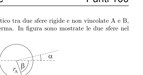
In una regione priva del campo di gravità si consideri l’urto elastico tra due sfere rigide e non vincolate A e B, di raggi rispettivamente $r_A$ e $r_B$, di cui una (B) inizialmente ferma. In figura sono mostrate le due sfere nel piano contenente i due centri e il vettore ${\vec{v}}_A$.

Siano $b$ il parametro d’impatto (definito come la distanza tra due rette passanti per i centri delle sfere e parallele a ${\vec{v}}_A$), $\alpha$ l’angolo di cui devia A e $\beta$ l’angolo tra la congiungente i due centri al momento dell’impatto e la traiettoria iniziale di A. Si misuri l’angolo $\alpha$ in verso antiorario e l’angolo $\beta$ in verso orario, in modo che entrambi risultino positivi come nella figura: pertanto $0^{\circ }\le \alpha \le 180^{\circ }$.

Si vuole determinare la massima deviazione angolare ${\alpha }_{\text{max}}$ che può subire A al variare del parametro d’impatto ($0\le b\le r_A+r_B$), in funzione della sua velocità iniziale e del rapporto tra le masse $\mu =m_A/m_B$.

Si supponga poi che l’attrito sia trascurabile e che quindi le forze impulsive al momento dell’impatto siano dirette lungo la congiungente i due centri.

1. Si dica quali tra le seguenti grandezze si conservano in questo tipo di urto, motivando la risposta: energia cinetica del sistema delle due sfere, energia cinetica della sfera A, quantità di moto totale, quantità di moto della sfera A.

Si consideri prima l’urto centrale, ovvero quello per $b=0$, per ogni valore di $\mu$ tra 0 e infinito.

2. Si scrivano le equazioni delle leggi di conservazione appropriate e si trovi la velocità $v_A^{\prime }$ della sfera A dopo l’urto.

Si passa adesso a studiare il caso generico con parametro d’impatto $b$ qualunque.

3. Qual è la massima deviazione, ${\alpha }_{\text{max}}$, al variare del parametro d’urto $b$, nel caso $\mu <1$ ?

Per le domande da 4. a 6., si consideri il caso $\mu \ge 1$, ponendo $s=\text{sen}\beta =b/(r_A+r_B)$.

4. Si scrivano le equazioni che descrivono le leggi di conservazione appropriate.

Si può dimostrare che nel caso generale che si sta esaminando vale la relazione

$\text{tg}\alpha =\frac{2s\sqrt{1-s^2}}{2s^2+\mu -1}.(1)$

5. Si dimostri che, nel caso $\mu =1$ le traiettorie delle due sfere, dopo l’urto, sono ortogonali.

6. Si ricavi qual è, al variare di $s$, la deviazione massima ${\alpha }_{\text{max}}$, per $\mu >1$, e la si esprima in funzione di $\mu$.

7. Si tracci il grafico di ${\alpha }_{\text{max}}$ in funzione di $\mu$.

p.4 — Urto tra due sfere rigide

Topic: Newtonian Mechanics, Conservation of Momentum, Conservation of Energy Metodi: Conservation of Momentum, Vector Decomposition, Kinematic Equations Competenze: Mathematical Modeling, Physical Reasoning, Diagrammatic Reasoning Objects: Sphere Fonte: Testo (PDF) — p.4 Soluzione: Soluzioni (PDF)

P1 Elastic scattering between two spheres 100 points

In a region free of gravity field, the elastic impact between two rigid, unbound spheres A and B, of radii $r_A$ and $r_B$ respectively, of which one (B) is initially stationary, is considered. The two spheres in the plane containing the two centres and the ${\vec{v}}_A$ vector are shown in Figure 1.

Siano $b$ il parametro d’impatto (definito come la distanza tra due rette passanti per i centri delle sfere e parallele a ${\vec{v}}_A$), $\alpha$ l’angolo di cui devia A e $\beta$ l’angolo tra la congiungente i due centri al momento dell’impatto e la traiettoria iniziale di A. The angle $\alpha$ is measured clockwise and the angle $\beta$ is measured clockwise, so that both are positive as shown in Figure: therefore $0^{\circ }\le \alpha \le 180^{\circ }$.

The maximum angular deviation ${\alpha }_{\text{max}}$ that A can experience when the impact parameter ($0\le b\le r_A+r_B$) varies, according to its initial velocity and the mass ratio $\mu =m_A/m_B$, is to be determined.

Suppose then that friction is negligible and that the impulsive forces at the time of impact are directed along the junction of the two centres.

1. Let’s say which of the following quantities are stored in this type of impact, which motivates the answer: kinetic energy of the two-sphere system, kinetic energy of the A-sphere, total motion quantity, amount of motion of the A-sphere.

Consider first the central impact, i.e. the one for $b=0$, for each value of $\mu$ between 0 and infinity.

2. Write the equations of the appropriate conservation laws and find the speed $v_A^{\prime }$ of the sphere A after impact.

Si passa adesso a studiare il caso generico con parametro d’impatto $b$ qualunque.

3. What is the maximum deviation, ${\alpha }_{\text{max}}$, from the change in the impact parameter $b$ in the case of $\mu <1$?

For the questions of four. a. 6., the case $\mu \ge 1$ is considered, and $s=\text{sen}\beta =b/(r_A+r_B)$ is inserted.

4. Write the equations that describe the appropriate conservation laws.

It can be shown that the general case under review is the report

$\text{tg}\alpha =\frac{2s\sqrt{1-s^2}}{2s^2+\mu -1}.(1)$

5. It is shown that in the case of $\mu =1$ the trajectories of the two spheres after impact are orthogonal.

6. The maximum deviation ${\alpha }_{\text{max}}$ for $\mu >1$ is obtained from $s$ and is expressed as a function of $\mu$.

7. The graph of ${\alpha }_{\text{max}}$ is plotted as a function of $\mu$.

**p.4 ** Collision between two rigid spheres

Topic: Newtonian Mechanics, Conservation of Momentum, Conservation of Energy Metodi: Conservation of Momentum, Vector Decomposition, Kinematic Equations Competenze: Mathematical Modeling, Physical Reasoning, Diagrammatic Reasoning Objects: Sphere Fonte: Testo (PDF) — p.4 Soluzione: Soluzioni (PDF)

P2 Modelli di atmosfera — Punti 100

In meteorologia si chiama “massa d’aria” una porzione di troposfera(1) di notevole estensione sia in orizzontale (anche molte decine di chilometri) che in verticale (una decina di chilometri) nella quale le grandezze termodinamiche come temperatura, pressione e umidità sono sostanzialmente uniformi ad una quota fissata.

L’atmosfera evolve nel tempo, ma tale evoluzione normalmente è lenta, e una massa d’aria può spostarsi orizzontalmente nell’atmosfera, mantenendo le sue caratteristiche, salvo il caso di fenomeni molto violenti come temporali e uragani, innescati da moti verticali di parti di essa. È importante osservare che quando una certa quantità d’aria relativamente piccola (per estensioni di decine di metri) viene perturbata e comincia a spostarsi verticalmente, questa può considerarsi termicamente isolata dal resto della massa d’aria, a causa del coefficiente di conduzione molto basso. Nel seguito una tale porzione, avente una massa definita, sarà denominata “cella”.

Per descrivere lo stato di equilibrio indifferente dell’intera massa d’aria, cioè la condizione per cui una qualunque cella perturbata e spostata verticalmente resta in equilibrio nella nuova posizione, si vogliono utilizzare due modelli, macroscopico e microscopico, confrontandone poi i risultati.

Dal punto di vista macroscopico, il modello più semplice è quello di un gas perfetto biatomico di massa molare media $\mu$, trascurando la presenza del vapore d’acqua, la variazione dell’accelerazione di gravità $g$ con la quota sul livello del mare $z$ ed effetti dovuti alla radiazione solare.

1. Preliminarmente, detta $p_0$ la pressione al livello del mare, si calcoli l’andamento della pressione con la quota, ovvero $p(z)$, in condizioni di equilibrio idrostatico, facendo l’ulteriore ipotesi che la temperatura sia uniforme e pari a $T_0$.

Nell’esecuzione dei calcoli si raccomanda di introdurre la costante $\lambda =R{T}_0/(\mu g)$.

2. La condizione di temperatura uniforme della massa d’aria è tale che l’equilibrio di una cella non possa essere indifferente; si dica se si tratta di equilibrio stabile o instabile, dandone una giustificazione qualitativa.

Applicando ancora il modello macroscopico termodinamico di gas perfetto biatomico, si consideri adesso il caso in cui la massa d’aria ha ancora pressione $p_0$ e temperatura $T_0$ al livello del mare, ma una temperatura $T$ variabile con la quota $z$ e tale che in essa ogni cella risulti in equilibrio indifferente.

3. Si calcoli l’andamento della temperatura $T(z)$ nella massa d’aria che consente ad una cella (isolata termicamente) di rimanere in equilibrio indifferente ad ogni quota.

Facendo uso adesso di un modello microscopico, si consideri per semplicità l’atmosfera come costituita da una sola specie di molecole (azoto $N_2$, di massa molare $\mu =28{\text{g mol}}^{-1}$). Le molecole sono in moto di agitazione termica e in condizioni di equilibrio. Si fa l’ipotesi che, grazie alle continue collisioni con altre molecole, l’energia totale media di ogni molecola sia indipendente dalla quota.

4. Calcolare l’andamento di temperatura con la quota, $T(z)$, secondo questo modello microscopico.

5. Utilizzando gli andamenti della temperatura ottenuti ai punti precedenti, si ricavi l’andamento della pressione, $p(z)$, per ciascuno dei due modelli.

6. Si dica in quali condizioni il caso elementare, discusso al punto 1, dà risultati convergenti con questi due modelli.

7. Per tutti e tre i casi studiati sopra, si calcolino i valori della pressione e della temperatura alla quota di 1000 m, se $p_0=100\text{kPa}$ e $T_0=20{}^{\circ }\text{C}$.

NOTE: 1. Può essere utile il seguente integrale indefinito:

$\int \frac{dx}{a+bx}=\frac{1}{b}\ln (a+bx)+\text{costante}.$

2. Possono tornare utili le seguenti approssimazioni valide se $x\ll 1$:

$e^x\approx 1+x$ $(1+x{)}^{\alpha }\approx 1+\alpha x.$

(1) La troposfera è la parte di atmosfera che si estende fino a circa 15 km di quota (alle nostre latitudini) in cui la ionizzazione è trascurabile.

Topic: Thermodynamics, Fluid Mechanics, Kinetic Theory Metodi: Hydrostatic Equilibrium, Ideal Gas Law, Kinetic Theory of Gases, Approximation & Series Expansion Competenze: Mathematical Modeling, Physical Reasoning, Estimation & Approximation Objects: Gas Fonte: Testo (PDF) — p.5 Soluzione: Soluzioni (PDF)

P2 Atmospheric patterns Points 100

In meteorology, a portion of the troposphere [1] of considerable extent is called “air mass” (or “air mass”) both horizontally (also many tens of kilometers) and vertically (one dozen kilometers) in which thermodynamic quantities such as temperature, pressure and humidity are essentially uniform at a fixed altitude.

The atmosphere evolves over time, but this evolution is normally slow, and a mass of air can move horizontally in the atmosphere, maintaining its characteristics, except for very violent phenomena such as storms and hurricanes, triggered by vertical motions of parts of it. It is important to note that when a certain amount of relatively small air (for extensions of tens of meters) is disturbed and begins to move vertically, this can be considered thermally isolated from the rest of the air mass, due to the very low conduction coefficient. In the following, such a portion, having a defined mass, shall be referred to as a ‘cell’.

To describe the state of indifferent equilibrium of the entire air mass, i.e. the condition in which any disrupted and vertically shifted cell remains in equilibrium in the new position, two models, macroscopic and microscopic, are to be used, and then the results are compared.

From a macroscopic point of view, the simplest model is that of a perfect biatomic gas of mean molar mass $\mu$, ignoring the presence of water vapor, the variation in gravitational acceleration $g$ with sea level elevation $z$ and effects due to solar radiation.

1. Initially, the pressure at sea level $p_0$ is calculated by the pressure trend with the quota, or $p(z)$, under hydrostatic equilibrium conditions, assuming that the temperature is uniform and equal to $T_0$.

It is recommended to enter the constant $\lambda =R{T}_0/(\mu g)$ when performing the calculations.

2. The uniform temperature condition of the air mass is such that the balance of a cell cannot be indifferent; whether it is a stable or unstable balance can be said, given a qualitative justification.

Applying the thermodynamic macroscopic model of perfect biatomic gas again, consider now the case where the air mass still has pressure $p_0$ and temperature $T_0$ at sea level, but a temperature $T$ variable with the quota $z$ and such that in it each cell is in an unbalanced state.

3. The temperature trend $T(z)$ in the air mass is calculated to allow a cell (thermically insulated) to remain in an unbalanced equilibrium at any altitude.

Using a microscopic model, the atmosphere is simply considered to consist of a single species of molecules (nitrogen $N_2$, molar mass $\mu =28{\text{g mol}}^{-1}$). The molecules are in thermal agitation and in equilibrium. It is assumed that, due to continuous collisions with other molecules, the average total energy of each molecule is independent of the height.

4. Calculate the temperature trend with the height, $T(z)$, according to this microscopic model.

5. Using the temperature trends obtained in the preceding points, the pressure trends, $p(z)$, are obtained for each of the two models.

6. The basic case, discussed in point 1, gives convergent results with these two models under what conditions.

7. For all three cases considered above, the pressure and temperature values at 1000 m altitude shall be calculated if $p_0=100\text{kPa}$ and $T_0=20{}^{\circ }\text{C}$.

The following is the list of the products: The following indefinite integer may be useful:

$\int \frac{dx}{a+bx}=\frac{1}{b}\ln (a+bx)+\text{costante}.$

2. The following valid approximations may be useful if $x\ll 1$:

$e^x\approx 1+x$ $(1+x{)}^{\alpha }\approx 1+\alpha x.$

(1) The troposphere is the part of the atmosphere that extends up to about 15 km of altitude (at our latitudes) where ionization is negligible.

Topic: Thermodynamics, Fluid Mechanics, Kinetic Theory Metodi: Hydrostatic Equilibrium, Ideal Gas Law, Kinetic Theory of Gases, Approximation & Series Expansion Competenze: Mathematical Modeling, Physical Reasoning, Estimation & Approximation Objects: Gas Fonte: Testo (PDF) — p.5 Soluzione: Soluzioni (PDF)

P3 Un sistema stellare binario — Punti 50

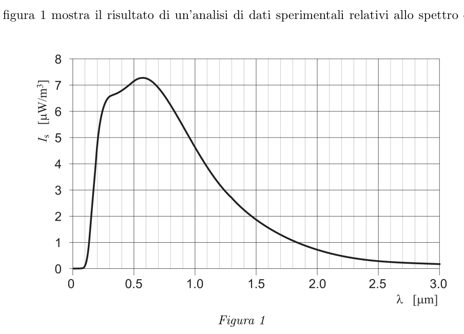
Il grafico di figura 1 mostra il risultato di un’analisi di dati sperimentali relativi allo spettro di una sorgente stellare.

Figura 1

In ordinata è riportata la quantità $I_s(\lambda )=dE/(dSdtd\lambda )$, detta “irradianza spettrale”, dove $dE$ è la quantità di energia, nell’intervallo di lunghezza d’onda $d\lambda$, che incide su una superficie $dS$ disposta perpendicolarmente alla direzione di propagazione della radiazione, in un intervallo di tempo $dt$.

In questo problema ogni stella sarà modellizzata come un corpo nero che emette radiazione alla temperatura superficiale della stella, uniforme sulla sua intera superficie.

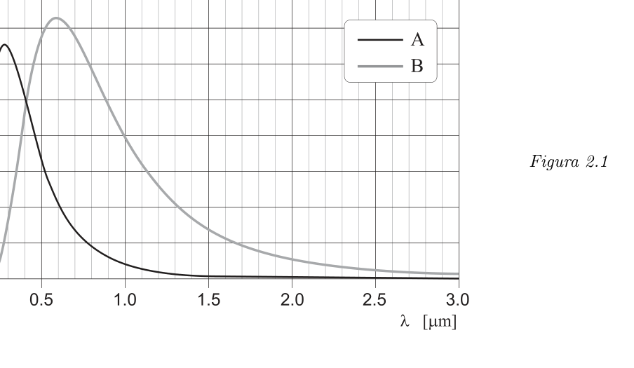
Il grafico di figura 1 non corrisponde a quello di un unico corpo nero. D’altra parte, una buona parte delle sorgenti stellari sono in realtà sistemi costituiti da due stelle, che orbitano l’una attorno all’altra. Molte di queste stelle doppie appaiono al telescopio come stelle singole solo perché sono troppo distanti dalla Terra per poter essere risolte. Si può quindi provare a vedere se questo spettro può essere ricavato come la sovrapposizione di due spettri di corpo nero distinti, corrispondenti a due stelle, indicate con le lettere A e B.

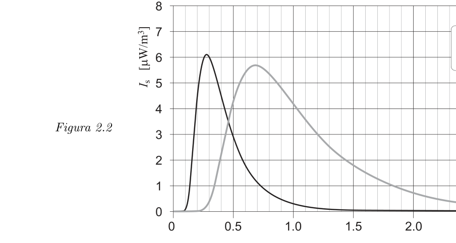
1. Individuare, motivando la risposta, quale delle coppie di spettri mostrate nella figura 2 (2.1 e 2.2) ha come somma lo spettro mostrato nella figura 1.

Figura 2.1

Figura 2.2

2. Ricavare le temperature superficiali delle due stelle A e B.

Senza fare alcun calcolo, si può vedere chiaramente che una delle due stelle è molto più luminosa dell’altra (in astronomia, con il termine “luminosità” ($L$) ci si riferisce alla potenza irraggiata dalla stella a tutte le lunghezze d’onda, non soltanto nell’intervallo del visibile).

3. Indicare, motivando la risposta, quale delle due stelle A e B è più luminosa.

Per determinare la distanza dalla Terra del sistema stellare in esame si può ricorrere al metodo della parallasse stellare, il quale sfrutta il cambiamento di posizione assunto dalla Terra durante il suo moto orbitale.

La tecnica presuppone la conoscenza del diametro dell’orbita terrestre e richiede più osservazioni dello stesso oggetto celeste per determinarne lo spostamento apparente rispetto allo sfondo.

La distanza angolare tra le posizioni estreme, raggiunte dal sistema stellare a sei mesi di distanza, è pari ad $\alpha =0.00204^{\prime \prime }$ (secondi d’arco).

4. Determinare la distanza del sistema stellare dalla Terra, in unità astronomiche (UA).

La figura 3 riporta lo spettro della stella A, ingrandito.

Figura 3

5. Calcolare, con un’incertezza massima del 15 %, la luminosità della stella A.

6. Calcolare il raggio della stella A.

7. Determinare, motivando la risposta, quale tra le due stelle A e B ha raggio maggiore.

p.6 — Irradianza spettrale in funzione di lambda

p.6 — Curve A e B, figura 2.1

p.7 — Curve A e B, figura 2.2

p.7 — Irradianza spettrale, figura 3

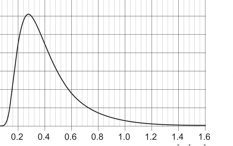
Topic: Astrophysics, Modern-Quantum Physics, Thermodynamics Metodi: Experimental Data Analysis, Physical Modeling, Graph Linearization Competenze: Physical Reasoning, Mathematical Modeling, Experimental Data Analysis Objects: Star Fonte: Testo (PDF) — p.6 Soluzione: Soluzioni (PDF)

P3 A binary star system Points 50

The graph in Figure 1 shows the result of an analysis of experimental data relating to the spectrum of a star source.

The following is the list of the following:

The quantity $I_s(\lambda )=dE/(dSdtd\lambda )$, called ‘spectral irradiance’, where $dE$ is the quantity of energy, in the wavelength range $d\lambda$, that affects a surface $dS$ perpendicular to the direction of radiation propagation, in a time range $dt$, is reported in order.

In this problem, each star will be modeled as a black body that emits radiation to the surface temperature of the star, uniform across its entire surface.

The graph in Figure 1 does not correspond to that of a single black body. On the other hand, a good part of the starry sources are actually systems of two stars orbiting each other. Many of these double stars appear as single stars to the telescope only because they are too far away from Earth to be solved. It can then be tested to see if this spectrum can be obtained as the superposition of two distinct black-body spectra, corresponding to two stars, indicated by letters A and B.

1. Identify, by reasoning the answer, which of the spectrum pairs shown in Figure 2 (2.1 and 2.2) sums up the spectrum shown in Figure 1.

The following table shows the following:

The following table shows the following:

2. Find the surface temperatures of the two stars A and B.

Without any calculation, one can clearly see that one of the two stars is much brighter than the other (in astronomy, the term “luminosity” ($L$) refers to the power radiated by the star at all wavelengths, not just in the range of the visible).

3. Indicate, motivating the answer, which of the two stars A and B is brighter.

To determine the distance from Earth of the star system under consideration, the method of stellar parallelism can be used, which exploits the change in position taken by the Earth during its orbital motion.

The technique assumes knowledge of the diameter of the Earth’s orbit and requires more observations of the same celestial object to determine its apparent displacement from the background.

The angular distance between the extreme positions, reached by the star system at six months’ distance, is $\alpha =0.00204^{\prime \prime }$ (arc seconds).

4. Determine the distance of the star system from the Earth, in astronomical units (UA).

Figure 3 shows the spectrum of star A, enlarged.

Figure 3

5. Calculate, with a maximum uncertainty of 15%, the brightness of star A.

6. Calculate the radius of star A.

7. Determine, motivating the answer, which of the two stars A and B has the greatest radius.

The following is the list of the parameters used for the calculation of the emission limit values:

The following table shows the results of the calculation of the total value of the assets:

The following table shows the results of the calculation of the total value of the assets:

The following is the list of the types of radiation used:

Topic: Astrophysics, Modern-Quantum Physics, Thermodynamics Metodi: Experimental Data Analysis, Physical Modeling, Graph Linearization Competenze: Physical Reasoning, Mathematical Modeling, Experimental Data Analysis Objects: Star Fonte: Testo (PDF) — p.6 Soluzione: Soluzioni (PDF)

P4 Due fili paralleli carichi — Punti 50

Su due fili isolanti – rettilinei, paralleli e di lunghezza infinita, a distanza $2a$ uno dall’altro – sono disposte cariche di segno opposto con densità lineare $\pm \lambda$ uniforme.

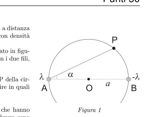
Si consideri, su un piano perpendicolare ai fili rappresentato in figura, la circonferenza di raggio $a$ passante per le intersezioni con i due fili, come in figura 1.

1. Calcolare il modulo del campo elettrico in ogni punto P della circonferenza (esclusi i punti di intersezione con i fili) e dire in quali punti è minimo.

2. Dimostrare che le due semicirconferenze di centro O che hanno come estremi le intersezioni dei fili con il piano della figura sono due linee di campo.

Figura 1

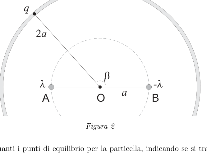
Una particella di carica positiva $q$ e massa $m$ è vincolata a muoversi su una guida circolare di raggio $2a$ complanare e concentrica alla circonferenza precedente (v. figura 2). La guida è costituita da un materiale isolante e la particella può scorrervi sopra con attrito trascurabile.

Figura 2

3. Determinare tutti quanti i punti di equilibrio per la particella, indicando se si tratta di equilibrio stabile o instabile.

4. La particella, posta inizialmente nel punto di equilibrio instabile viene spostata di una piccola quantità e lasciata libera. Determinare la velocità della particella quando passa per il punto di equilibrio stabile.

I due fili si muovono ora entrambi con velocità $\vec{v}$ parallela ai fili stessi.

5. Dimostrare che in ogni punto il campo magnetico $\vec{B}$ è perpendicolare al campo elettrico $\vec{E}$ e tra i moduli dei campi vale la relazione $B=vE/c^2$ (ovvero $vB=(v/c{)}^{2}E$).

p.8 — Due fili carichi e circonferenza, figura 1

p.8 — Geometria fili e circonferenza, figura 2

Topic: Electrostatics, Magnetism, Newtonian Mechanics Metodi: Gauss’s Law, Coulomb’s Law, Energy Conservation Method, Free-Body Diagram Competenze: Mathematical Modeling, Diagrammatic Reasoning, Physical Reasoning Objects: Wire, Point Charge Fonte: Testo (PDF) — p.8 Soluzione: Soluzioni (PDF)

P4 Two parallel wires loaded Points 50

On two insulating wires straight, parallel and infinite length, at a distance $2a$ from each other opposite sign loads with uniform linear density $\pm \lambda$ are arranged.

Consider, on a plane perpendicular to the wires shown in Figure 1, the radius circumference $a$ passing through the intersections with the two wires, as shown in Figure 1.

1. Calculate the electric field modulus at each point P of the circumference (excluding the points of intersection with the wires) and tell which points is the minimum.

2. To show that the two semicircular centre O which have as their extremes the intersections of the strings with the plane of the figure are two field lines.

The following is the list of the following:

A positive charge particle $q$ and mass $m$ is bound to move on a circular guide of radius $2a$ flat and concentric to the previous circumference (see paragraphs 1 and 2). The Commission shall adopt implementing acts in accordance with Article 21 of this Regulation. The guide is made of an insulating material and the particle can run over it with negligible friction.

Figure 2

3. Determine all the equilibrium points for the particle, indicating whether it is stable or unstable.

4. The particle, initially placed at the point of unstable equilibrium, is moved a small amount and left free. Determine the velocity of the particle as it passes through the stable equilibrium point.

The two wires are now moving both at $\vec{v}$ speed parallel to the wires themselves.

5. Show that at each point the magnetic field $\vec{B}$ is perpendicular to the electric field $\vec{E}$ and that the ratio between the modules of the fields is $B=vE/c^2$ (i.e. $vB=(v/c{)}^{2}E$).

**p.8 ** Two wires loaded and circumference, figure 1

The following table shows the number of lines of reference for each line of the reference line:

Topic: Electrostatics, Magnetism, Newtonian Mechanics Metodi: Gauss’s Law, Coulomb’s Law, Energy Conservation Method, Free-Body Diagram Competenze: Mathematical Modeling, Diagrammatic Reasoning, Physical Reasoning Objects: Wire, Point Charge Fonte: Testo (PDF) — p.8 Soluzione: Soluzioni (PDF)