OII na Nazionale Teorica

P1 Il fischio del treno Punti 100 Una sorgente sonora S, in moto a velocità costante $v$, emette un segnale, a frequenza $f_0$; un sensore ne misura la frequenza $f$. Si assuma per la velocità del suono $c=340{\text{m s}}^{-1}$, maggiore di quella della sorgente.

1. Quale frequenza $f$ verrà registrata da un sensore fermo in un punto P di fronte alla sorgente se questa gli sta andando incontro lungo la congiungente SP? Più in generale, il sensore è posto in un punto P, molto lontano dalla sorgente, tale che la direzione SP formi un angolo $\phi$ con la velocità della sorgente stessa.
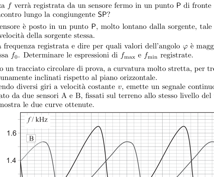
2. Determinare la frequenza registrata e dire per quali valori dell’angolo $\phi$ è maggiore, minore o uguale alla frequenza emessa $f_0$. Determinare le espressioni di $f_{\text{max}}$ e $f_{\text{min}}$ registrate. Si sta sperimentando un tracciato circolare di prova, a curvatura molto stretta, per treni ad alta velocità, in cui i binari sono opportunamente inclinati rispetto al piano orizzontale. Il treno, percorrendo diversi giri a velocità costante $v$, emette un segnale continuo a frequenza costante $f_0$; questo viene registrato da due sensori A e B, fissati sul terreno allo stesso livello del tracciato di prova, avente raggio $r$. Il grafico mostra le due curve ottenute. Nel seguito, le risposte dovranno essere accompagnate da una rappresentazione grafica della situazione in esame, avendo fissato un sistema di riferimento cartesiano piano con origine nel centro O del tracciato di raggio $r$. Per iniziare, si scelga l’asse $x$ lungo la congiungente del centro con la posizione del sensore A e si assumano per A le coordinate $(a,0)$, con $a>r$.
3. Determinare la massima frequenza registrata dal sensore A, in funzione di $r$, $a$ ed $f_0$ e, sul piano cartesiano, indicare con $M_1$ il punto del tracciato circolare in cui si trovava il treno nel momento in cui emetteva il segnale che, dopo un certo ritardo, è stato ricevuto con la frequenza massima. Analogamente, per la minima frequenza, indicare il punto $M_2$. Riportare chiaramente nel disegno i parametri $r$ e $a$, indicando con $\alpha$ l’angolo $\widehat{M_{1}OA}$.
4. Dal grafico precedente, che riporta la registrazione dei due sensori, ricavare la frequenza $f_0$ del segnale emesso dal treno e la velocità $v$ del treno.
5. Calcolare il raggio $r$ del tracciato circolare e le distanze $a=OA$ e $M_{1}A$, spiegando perché, in questo caso, si può ignorare il tempo di ritardo di propagazione del segnale sonoro.
6. Spiegare perché il sensore B è certamente posto all’interno del tracciato del treno. In una seconda figura, relativa al sensore B, disegnare un piano cartesiano analogo al precedente, in cui il sensore B è posto in $(b,0)$ con $b<r$. Si determinino le espressioni della frequenza massima e minima registrata dal sensore B in funzione di $f_0$, $r$ e della sua distanza $b$ dal centro O del tracciato, riportando poi i punti $N_1$ e $N_2$ corrispondenti alle due posizioni del treno definite come sopra. Indicare con $\beta$ l’angolo $\widehat{N_{1}OB}$.
7. Si calcolino le distanze $b=OB$ e $N_{1}B$.
8. Utilizzando adesso un unico piano cartesiano, sul quale il sensore A sta di nuovo in $(a,0)$, dopo aver determinato l’angolo $\theta =\widehat{M_{1}O{N}_1}$, si riporti la corretta posizione del sensore B rispetto ad A e si calcoli la distanza $L$ tra di essi.

p.3 — Grafico della frequenza registrata nel tempo

Topic: Oscillations & Waves, Newtonian Mechanics Metodi: Wave Equation, Kinematic Equations, Experimental Data Analysis, Vector Decomposition Competenze: Mathematical Modeling, Diagrammatic Reasoning, Experimental Data Analysis Objects: — Fonte: Testo (PDF) — p.3 Soluzione: Soluzioni (PDF)

P1 The train whistle The following points shall be added: A sound source S, moving at constant speed $v$, emits a signal, at frequency $f_0$; a The sensor measures the frequency $f$. It is assumed that the sound speed $c=340{\text{m s}}^{-1}$ is greater than that of the The source.

1. What frequency $f$ will be recorded by a stationary sensor at a point P in front of the source if this is the Is he going to meet along the SP junction? More generally, the sensor is placed at a point P, very far from the source, such that the SP direction forms a $\phi$ angle with the speed of the source itself.
2. Determine the recorded frequency and tell which values of the angle $\phi$ is greater, less or equal to The frequency of emission $f_0$. Determine the recorded expressions of $f_{\text{max}}$ and $f_{\text{min}}$. We are experimenting with a very narrow-circle test track for high-speed trains, where the tracks are properly tilted relative to the horizontal plane. The train, running several laps at constant speed $v$, shall transmit a continuous signal at constant frequency $f_0$; This is recorded by two sensors A and B, fixed to the ground at the same level as the test track, having The radius $r$. The graph shows the two curves obtained. The following answers shall be accompanied by a graphic representation of the situation under consideration, having a flat Cartesian reference system originating in the centre O of the $r$ radius path. For to start, select the $x$ axis along the centre junction with the sensor position A and assume for A the coordinates $(a,0)$, with $a>r$.
3. Determine the maximum frequency recorded by sensor A, according to $r$, $a$ and $f_0$ and, on the Cartesian plane, indicate with $M_1$ the point of the circular track where the train was at the time of the emission of the The signal that, after some delay, has been received at maximum frequency. Similarly, for the minimum frequency, indicate the point $M_2$. Clearly report the parameters $r$ and $a$ in the drawing, indicating with $\alpha$ the angle $\widehat{M_{1}OA}$.
4. From the previous graph, which shows the recording of the two sensors, obtain the $f_0$ frequency of the signal the train is emitted and the train speed $v$.
5. Calculate the radius $r$ of the circular path and the distances $a=OA$ and $M_{1}A$, explaining why, in this case, the delay in propagation of the sound signal can be ignored.
6. Explain why the B sensor is certainly placed inside the train track. In a second figure, for sensor B, draw a map map similar to the previous one, in which the sensor B is placed in $(b,0)$ con $b<r$. Determine the maximum and minimum frequency expressions recorded by the sensor B in the function of $f_0$, $r$ and its distance $b$ from the centre O of the track, then returning the points $N_1$ and $N_2$ corresponding to the two train positions defined as above. The angle $\widehat{N_{1}OB}$ shall be indicated with $\beta$.
7. The distances $b=OB$ and $N_{1}B$ shall be calculated.
8. Utilizzando adesso un unico piano cartesiano, sul quale il sensore A sta di nuovo in $(a,0)$, dopo aver The angle $\theta =\widehat{M_{1}O{N}_1}$ is determined, the correct position of the sensor B is returned to A and the The distance $L$ between them.

**p.3 ** Time-recorded frequency chart

Topic: Oscillations & Waves, Newtonian Mechanics Metodi: Wave Equation, Kinematic Equations, Experimental Data Analysis, Vector Decomposition Competenze: Mathematical Modeling, Diagrammatic Reasoning, Experimental Data Analysis Objects: — Fonte: Testo (PDF) — p.3 Soluzione: Soluzioni (PDF)

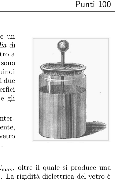
P2 Tre-in-uno Punti 100 A - La Bottiglia di Leida Agli albori della ricerca sull’elettricità (circa 1750) si conosceva solamente un dispositivo per “immagazzinare” l’energia elettrica, conosciuto come bottiglia di Leida, dal nome dell’omonima città olandese. Questo è un contenitore in vetro a forma cilindrica sulle cui superfici interne ed esterne, compresa la base, sono applicati dei fogli di alluminio. Come in un condensatore piano si hanno quindi due superfici metalliche isolate l’una dall’altra. In questo caso la distanza tra i due piani sarà semplicemente lo spessore del vetro, molto sottile, per cui le superfici metalliche interne ed esterne sono da considerarsi praticamente identiche e gli effetti di bordo possono essere trascurati. Si consideri la seguente bottiglia di Leida: il contenitore è stato ricoperto all’interno e all’esterno con fogli di alluminio per un’altezza $h=18.0\text{cm}$ e, analogamente, è stato ricoperto il fondo circolare che ha raggio $r=4.2\text{cm}$. Lo spessore del vetro è $d=2.0\text{mm}$. La costante dielettrica del vetro di questa bottiglia è ${\epsilon }_r=8.1$.

1. Calcolare la capacità $C$ di questa bottiglia di Leida. La rigidità dielettrica è definita come il valore limite di campo elettrico $E_{\text{max}}$, oltre il quale si produce una conduzione di elettricità (scarica elettrica) attraverso il materiale dielettrico. La rigidità dielettrica del vetro è all’incirca $E_{\text{max}}=30\times 10^6{\text{V m}}^{-1}$.
2. Calcolare la carica massima $Q_{\text{max}}$ che può essere accumulata su questa bottiglia di Leida. Dopo aver caricato la bottiglia di Leida fino al massimo trovato sopra, si collegano le due superfici metalliche attraverso una resistenza $R=100\Omega$.
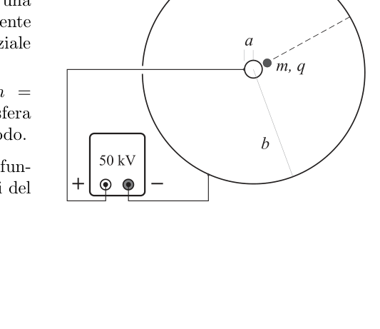
3. Dopo quanto tempo $t_E$ la bottiglia di Leida si sarà scaricata fino allo 0.10 % della carica iniziale? ——————————— B - Volo di una particella carica puntiforme L’apparato mostrato in figura – dove per chiarezza le proporzioni non sono rispettate – è costituito da una piccola sfera conduttrice di raggio $a=1\text{cm}$, caricata positivamente (anodo) al centro di una sfera molto più grande, di raggio $b=1\text{m}$, caricata negativamente (catodo). Tra le due sfere viene stabilita una differenza di potenziale $\Delta V=50\text{kV}$. Una particella carica, positiva e puntiforme, con $k=q/m=10^2{\text{C kg}}^{-1}$, mantenuta ferma in prossimità della superficie della sfera piccola, viene lasciata e inizia a muoversi nel vuoto verso il catodo.
4. Ricavare l’espressione della velocità $v$ della particella, in funzione della sua distanza $r$ dal centro del sistema e dei dati del problema.
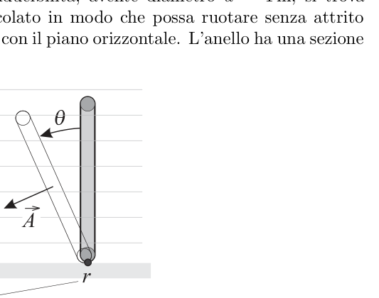
5. Determinare il tempo di volo della particella. ———————— Nella soluzione può servire il seguente integrale: $\int \frac{dx}{\sqrt{1-a/x}}=\sqrt{x(x-a)}+a\ln \left(\sqrt{x}+\sqrt{x-a}\right)+c\text{per}x>a>0.$ ——————————— — Pagina 4 di 8 — AIF – Campionati di Fisica 2026 Gara Nazionale – 17 aprile 2026 – Prova teorica C - Correnti indotte in anello che cade Un grande anello sottile di materiale conduttore di bassa conducibilità, avente diametro $d=1\text{m}$, si trova in posizione verticale su di un pavimento orizzontale ed è vincolato in modo che possa ruotare senza attrito attorno all’asse $r$ costituito dall’intersezione del piano dell’anello con il piano orizzontale. L’anello ha una sezione trasversale $S=1{\text{cm}}^2$. Essendo in equilibrio instabile, l’anello inizia a cadere. Nella regione dove si trova l’anello il campo magnetico terrestre può essere considerato orizzontale, rivolto nella direzione iniziale dell’asse dell’anello con un’intensità $B=50\mu \text{T}$.
6. Supponendo di poter trascurare gli effetti dovuti alla corrente indotta nell’anello, determinare il modulo della f.e.m. indotta in funzione dell’angolo $\theta$ tra il piano verticale e il piano dell’anello.
7. Sapendo che la resistività del conduttore è $\rho =0.2\mu \Omega \text{m}$, qual è il massimo valore della corrente $I$ circolante nell’anello mentre esso cade al suolo? Nelle domande precedenti si è trascurato il momento torcente dovuto al campo magnetico sulla spira percorsa da corrente.
8. Si giustifichi a posteriori questa affermazione, dando una stima quantitativa del rapporto fra i valori massimi dei moduli del momento magnetico e del momento meccanico – calcolati rispetto al punto di contatto – agenti sulla spira. Si ricorda che il momento d’inerzia di un anello sottile, rispetto a un asse diametrale, è $\frac{1}{2}M{R}^2$, dove $M$ è la massa e $R$ è il raggio. Sia $\delta =7.85\times 10^3{\text{kg m}}^{-3}$ la densità del materiale conduttore.

p.4 — Bottiglia di Leida cilindrica

p.4 — Particella carica in orbita circolare

p.5 — Anello carico che cade lungo asse

Topic: Electrostatics, Circuits, Electromagnetic Induction Metodi: Coulomb’s Law, Electric Potential Method, Conservation of Energy, Faraday’s Law of Induction Competenze: Mathematical Modeling, Physical Reasoning, Estimation & Approximation Objects: Capacitor, Resistor, Conducting Sphere, Point Charge, Wire Fonte: Testo (PDF) — p.4 Soluzione: Soluzioni (PDF)

P2 Three in one The following points shall be added: A - The Leida bottle At the dawn of electricity research (c. 1750) only one person was known. A device for storing electrical energy, known as a bottle of Leida, named after the Dutch city of the same name. This is a glass container cylindrical shape on which the inner and outer surfaces, including the base, are Applied with aluminium foil. As in a flat capacitor you have then two metal surfaces isolated from each other. In this case, the distance between the two The surface is very thin, so the surface is very thin. The internal and external metals are considered to be virtually identical and the the effects on board may be neglected. Consider the following Leida bottle: the container was covered inside and outside with aluminium foil for a height of $h=18.0\text{cm}$ and, similarly, the circular bottom with a radius $r=4.2\text{cm}$ has been covered. The thickness of the glass è $d=2.0\text{mm}$. The dielectric constant of the glass in this bottle is ${\epsilon }_r=8.1$.

1. Calculate the $C$ capacity of this bottle of Leida. Dielectric rigidity is defined as the electric field limit value $E_{\text{max}}$, above which an conduction of electricity (electric discharge) through dielectric material. The dielectric stiffness of the glass is all’incirca $E_{\text{max}}=30\times 10^6{\text{V m}}^{-1}$.
2. Calculate the maximum load $Q_{\text{max}}$ that can be accumulated on this bottle of Leida. After loading the Leida bottle to the top, the two metal surfaces are connected through a resistance $R=100\Omega$.
3. How long after $t_E$ has the Leida bottle been discharged up to 0.10% of the initial load? ——————————— B - Flight of a pointed-loaded particle The apparatus shown in Figure where the proportions are clearly It is made up of a small conductive sphere a radius $a=1\text{cm}$, positively charged (anode) at the centre of a a much larger sphere, with a radius $b=1\text{m}$, negatively charged (Catholic) The difference in potential between the two spheres is established. $\Delta V=50\text{kV}$. A positive, pointed particle with $k=q/m=10^2{\text{C kg}}^{-1}$, held firm near the surface of the sphere Little girl, she’s left and starts moving in the void towards the cathode.
4. The expression of the particle velocity $v$, based on its distance $r$ from the centre of the system and the data of the I’m not sure.
5. Determine the particle’s flight time. ———————— The solution may be served with the following integral: $\int \frac{dx}{\sqrt{1-a/x}}=\sqrt{x(x-a)}+a\ln \left(\sqrt{x}+\sqrt{x-a}\right)+c\text{per}x>a>0.$ ——————————— Page 4 of 8 AIF Physics Championships 2026 National competition 17 April 2026 Theoretical proof C - Induced ring currents A large thin ring of conductive material of low conductivity, with a diameter $d=1\text{m}$, is located It is positioned vertically on a horizontal floor and is bound so that it can rotate without friction around the $r$ axis consisting of the intersection of the plane of the ring with the horizontal plane. The ring has a section. trasversale $S=1{\text{cm}}^2$. Being in unstable equilibrium, the ring begins to fall. In the region where the ring is located the magnetic field The ground axis can be considered horizontal, facing in the initial direction of the ring axis with a $B=50\mu \text{T}$.
6. Assuming that the effects of induced current in the ring can be overlooked, determine the of the F.E.M. induced by the angle $\theta$ between the vertical plane and the plane of the ring.
7. Knowing that the resistance of the conductor is $\rho =0.2\mu \Omega \text{m}$, what is the maximum value of the current circulating $I$ In the ring as it falls to the ground? In the previous questions, the torque due to the magnetic field on the spindle was ignored. It’s electric.
8. This statement is later justified by a quantitative estimate of the ratio between the values of the Maximum of the magnetic moment and mechanical moment modules calculated from the point of Contact agents on the spire. It is recalled that the moment of inertia of a thin ring relative to a diameter axis is $\frac{1}{2}M{R}^2$, where $M$ is the mass and $R$ is the radius. The density of the conductive material shall be $\delta =7.85\times 10^3{\text{kg m}}^{-3}$.

p.4 — Bottiglia di Leida cilindrica

p.4 — Particella carica in orbita circolare

**p.5 ** Load ring that falls along the axis

Topic: Electrostatics, Circuits, Electromagnetic Induction Metodi: Coulomb’s Law, Electric Potential Method, Conservation of Energy, Faraday’s Law of Induction Competenze: Mathematical Modeling, Physical Reasoning, Estimation & Approximation Objects: Capacitor, Resistor, Conducting Sphere, Point Charge, Wire Fonte: Testo (PDF) — p.4 Soluzione: Soluzioni (PDF)

P3 Oscillazioni di un fluido Punti 100 Un fluido ideale (1), contenuto in un tubo a forma di U, si dispone in equilibrio come mostrato in figura 1, in presenza del campo gravitazionale. Siano $A$ la sezione trasversale del tubo, $\rho$ la densità del fluido, $L$ la lunghezza del tratto di tubo occupato dal fluido e $h<L/2$ la differenza di quota tra il tratto inferiore del tubo e i punti del fluido posti più in alto. In tutte le figure mostrate nel problema, le parti curve che raccordano i tratti dritti del tubo sono state esagerate per ragioni di chiarezza, ma, per tutto il problema, va supposto che il diametro del tubo sia molto minore delle lunghezze in gioco, in modo da poter descrivere i punti nel fluido tramite una sola coordinata. Tali parti curve, però, sono necessarie a evitare la formazione di turbolenze. (1) Nel problema per “fluido ideale” si intende un fluido incomprimibile, non viscoso e tale che si possa trascurare l’attrito con le pareti del condotto dove scorre. Si suppone inoltre che il fluido non scorra mai in regime turbolento.

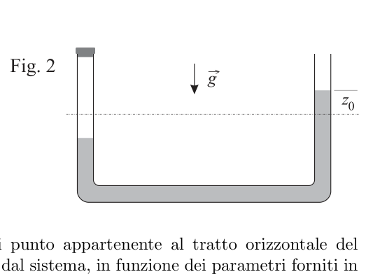
1. Quanto vale la pressione sul fondo del tubo in condizioni di equilibrio, come in figura 1, se $p_0$ è la pressione atmosferica? L’estremità sinistra del tubo viene tappata e, tramite una pompa d’aria, la pressione al suo interno viene aumentata fino al valore $p_1$. Di conseguenza, il fluido si sposta verso destra, innalzandosi di un tratto $z_0$ al di sopra del livello originario, ma senza raggiungere il bordo del tubo.
2. In riferimento alla nuova configurazione di equilibrio mostrata in figura 2, quanto vale $z_0$? Nel seguito utilizzare solo il parametro $z_0$ e non la sua espressione appena trovata.
3. Scegliendo come zero dell’energia potenziale un qualsiasi punto appartenente al tratto orizzontale del tubo, trovare l’energia potenziale gravitazionale posseduta dal sistema, in funzione dei parametri forniti in precedenza. Il tappo viene rimosso istantaneamente e, di conseguenza, il fluido inizia a muoversi. In un generico istante di tempo, sia $z(t)$ la quota del pelo libero di destra.
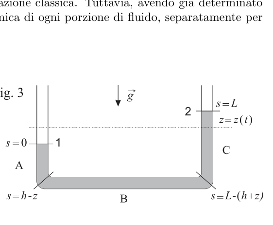
4. Trovare la legge oraria $z=z(t)$ che descrive il moto dell’estremità superiore destra del fluido, dove $t$ è misurato dall’istante in cui il tappo viene rimosso. La situazione appena studiata si riferisce a un fluido che non si trova in condizioni statiche né si muove in regime stazionario; di conseguenza per calcolare la pressione in ogni punto del fluido non si possono applicare né la legge di Stevino, né il teorema di Bernoulli nella sua formulazione classica. Tuttavia, avendo già determinato il moto d’insieme del fluido, sarà sufficiente studiare la dinamica di ogni porzione di fluido, separatamente per ognuna delle tre sezioni del tubo a U. In un generico istante di tempo $t$, si considerino i punti estremi del fluido (1 e 2 in figura 3) e si parametrizzino tutti i punti del fluido compresi tra questi tramite la coordinata $s$, che va da 0 (punto 1) a $L$ (punto 2).
5. Trovare l’andamento della pressione $p_z(s)$ in funzione di $s$ (tra $s=0$ e $s=L$), per ogni valore istantaneo di $z$.
6. Rappresentare graficamente, in modo qualitativo, l’andamento di $p_z(s)$ trovato al punto precedente, specificando in quali punti del tubo la pressione è massima, separatamente nei due casi $z>0$ e $z<0$. Nel caso in cui gli effetti viscosi non possano essere trascurati, c’è bisogno di apportare delle modifiche al modello. La viscosità si descrive introducendo una forza di attrito, dipendente dalla velocità media $⟨v⟩$ delle particelle del fluido: $F_v=8\pi \mu L⟨v⟩$ dove $\mu$ è il coefficiente di viscosità. Naturalmente, ci si aspetta che la nuova legge oraria $z(t)$ abbia un andamento smorzato, a causa della dissipazione di energia dovuta a tali effetti. Partendo da condizioni iniziali leggermente diverse dalle precedenti, si osserva un moto di questo tipo $z(t)=z_0\cos (\omega t)e^{-t/\tau }$ con $\tau$ tempo caratteristico di smorzamento.
7. Trovare il tempo caratteristico $\tau$ e la pulsazione $\omega$ del sistema oscillante in funzione della viscosità $\mu$ e degli altri parametri del problema. — Pagina 6 di 8 — AIF – Campionati di Fisica 2026 Gara Nazionale – 17 aprile 2026 – Prova teorica Tavola di Costanti Fisiche Costanti Fisiche Primarie [ Valori esatti per definizione – (26.CGPM/16.11.2018) ] COSTANTE SIMB. VALORE UNITÀ Velocità della luce nel vuoto $c$ $2.99792458\times 10^8$ ${\text{m s}}^{-1}$ Carica elementare $e$ $1.602176634\times 10^{-19}$ C Costante di Planck $h$ $6.62607015\times 10^{-34}$ J s Costante di Boltzmann $k$ $1.380649\times 10^{-23}$ ${\text{J K}}^{-1}$ Costante di Avogadro $N_A$ $6.02214076\times 10^{23}$ ${\text{mol}}^{-1}$ Costanti definite [ Valori esatti per convenzione ] Unità Astronomica [ 28.Ass. Gen. IAU (2012) ] au 149 597 870 700 m Accelerazione di gravità [ 3.CGPM (1901) ] $g$ 9.80665 ${\text{m s}}^{-2}$ Temperatura standard ($0{}^{\circ }\text{C}$) $T_0$ 273.15 K Pressione atmosferica standard $p_a$ $1.01325\times 10^5$ Pa Altre Costanti Fisiche [ Valori arrotondati con ${\epsilon }_r<10^{-5}$ ] † Massa dell’elettrone $m_e$ $9.1094\times 10^{-31}$ kg $=5.1100\times 10^2$ ${\text{keV c}}^{-2}$ Massa del protone $m_p$ $1.67262\times 10^{-27}$ kg $=9.3827\times 10^2$ ${\text{MeV c}}^{-2}$ Massa del neutrone $m_n$ $1.67493\times 10^{-27}$ kg $=9.3955\times 10^2$ ${\text{MeV c}}^{-2}$ Permeabilità magnetica del vuoto ${\mu }_0$ $1.25664\times 10^{-6}=4\pi \times 10^{-7}$ ${\text{H m}}^{-1}$ Costante dielettrica del vuoto: $1/({\mu }_0{c}^2)$ ${\epsilon }_0$ $8.8542\times 10^{-12}$ ${\text{F m}}^{-1}$ Costante elettrostatica: $1/(4\pi {\epsilon }_0)$ $k_{es}$ $8.9876\times 10^9=c^2\times 10^{-7}$ ${\text{m F}}^{-1}$ Costante universale dei gas: $N_{A}k$ $R$ 8.3145 ${\text{J mol}}^{-1}{\text{K}}^{-1}$ Costante di Faraday: $N_{A}e$ $F$ $9.6485\times 10^4$ ${\text{C mol}}^{-1}$ Costante di Stefan–Boltzmann $\sigma$ $5.6704\times 10^{-8}$ ${\text{W m}}^{-2}{\text{K}}^{-4}$ Costante di gravitazione universale $G$ $6.674\times 10^{-11}$ ${\text{m}}^3{\text{kg}}^{-1}{\text{s}}^{-2}$ Volume molare di un gas perfetto in condizioni standard ($p_a$, $T_0$) $V_m$ $2.2414\times 10^{-2}$ ${\text{m}}^3{\text{mol}}^{-1}$ Unità di massa atomica u $1.66054\times 10^{-27}$ kg Tavola di dati che possono essere necessari † Densità dell’acqua (a $4{}^{\circ }\text{C}$)⋆ ${\rho }_a$ $1.00000\times 10^3$ ${\text{kg m}}^{-3}$ Calore specifico dell’acqua (a $20{}^{\circ }\text{C}$)⋆ $c_a$ $4.182\times 10^3$ ${\text{J kg}}^{-1}{\text{K}}^{-1}$ Densità del ghiaccio (a $0{}^{\circ }\text{C}$)⋆ ${\rho }_{g,0}$ $0.917\times 10^3$ ${\text{kg m}}^{-3}$ Calore di fusione del ghiaccio ${\lambda }_f$ $3.344\times 10^5$ ${\text{J kg}}^{-1}$ Calore di vaporizzazione dell’acqua (a $100{}^{\circ }\text{C}$)⋆ ${\lambda }_v$ $2.257\times 10^6$ ${\text{J kg}}^{-1}$ † Da considerare esatti nella soluzione delle prove dei Campionati di Fisica. ⋆ Salvo diversa indicazione esplicita, questi dati si potranno utilizzare anche ad altre temperature senza errori importanti. — Pagina 7 di 8 — AIF – Campionati di Fisica 2026 Gara Nazionale – 17 aprile 2026 – Prova teorica NOTA BENE: È possibile utilizzare, riprodurre, distribuire, comunicare al pubblico questo materiale alle due seguenti condizioni: citare la fonte; non usare il materiale, nemmeno parzialmente, per fini commerciali. — Pagina 8 di 8 —

p.6 — Tubo a U con fluido spostato

p.6 — Tubo a U con secondo fluido

Topic: Fluid Mechanics, Oscillations & Waves Metodi: Hydrostatic Equilibrium, Differential Equations, Energy Conservation Method, Physical Modeling Competenze: Mathematical Modeling, Physical Reasoning, Diagrammatic Reasoning Objects: Tube Fonte: Testo (PDF) — p.5 Soluzione: Soluzioni (PDF)

P3 Fluid oscillations The following points shall be added: An ideal fluid (1), contained in a tube U-shaped, balanced as shown in Figure 1, In the presence of the gravitational field. The length of the tube is $A$, the fluid density $\rho$, the length of the tube $L$. The difference between the fluid and the fluid is $h<L/2$ the distance between the bottom of the tube and the fluid points placed higher up. In all the figures shown in the problem, the curved parts that The length of the tube is much smaller than the diameter of the tube. In the game, so you can describe the points in the fluid using a single coordinate. However, these curved parts are The Commission shall adopt implementing acts in accordance with the procedure referred to in Article 2 of Regulation (EC) No 1272/2003. (1) The problem for ‘ideal fluid’ means an incompressible, non-viscous fluid which can be neglected by friction with the walls of the conduit where it flows. It is also assumed that the fluid never flows in a turbulent mode.

1. What is the pressure on the bottom of the tube under equilibrium conditions, as shown in Figure 1, if $p_0$ is the pressure The atmosphere? The left end of the tube is closed and, by means of a The pressure inside the pump is increased. up to $p_1$. As a result, the fluid moves to the Right, rising slightly $z_0$ above the level originally, but without reaching the edge of the tube.
2. With reference to the new balance configuration As shown in Figure 2, what is $z_0$? Use only the $z_0$ parameter below and not your The expression just found.
3. The potential energy of the energy is determined by selecting any point in the horizontal line of the The system’s gravitational potential energy, based on the parameters provided in the The Commission has already taken a number of measures. The lid is removed instantly and, as a result, the fluid begins to move. In a general moment of time, be $z(t)$ the right hair share.
4. Find the $z=z(t)$ time law that describes the motion of the upper right end of the fluid, where $t$ is measured from the moment the lid is removed. The situation just studied refers to a fluid that is neither in static conditions nor moving in mode The pressure at each point of the fluid cannot be calculated by using either the The law of Stevino, nor the Bernoulli theorem in its classical formulation. However, having already determined that the The total movement of the fluid, it will be sufficient to study the dynamics of each fluid portion separately for Each of the three sections of the U tube. In a general moment of time $t$, consider the following: extreme points of the fluid (1 and 2 in Figure 3) and all points of the fluid included in these are parameterized by the coordinate $s$, which runs from 0 (point 1) to $L$ (point 2)
5. Find the pressure gradient $p_z(s)$ as a function of $s$ (between $s=0$ and $s=L$), for each value istantaneo di $z$.
6. Graphically represent the $p_z(s)$ trend found in the previous point, specifying at which points of the tube the pressure is maximum, separately in both cases $z>0$ e $z<0$. If the viscous effects cannot be overlooked, changes to the model. Viscosity is described by introducing a friction force, which depends on the mean speed $⟨v⟩$ of the Particles of the fluid: $F_v=8\pi \mu L⟨v⟩$ where $\mu$ is the viscosity coefficient. Of course, it is expected that the The new time law $z(t)$ has a dim trend, due to the energy dissipation due to these effects. Starting from slightly different initial conditions, a motor of this type is observed. $z(t)=z_0\cos (\omega t)e^{-t/\tau }$ with $\tau$ characteristic time of attenuation.
7. Find the characteristic time $\tau$ and pulse $\omega$ of the oscillating system depending on the viscosity $\mu$ and The Commission will examine the other parameters of the problem. Page 6 of 8 AIF Physics Championships 2026 National competition 17 April 2026 Theoretical proof Table of physical constants Primary physical constants The following table shows the total value of the assets of the Union industry as defined in Article 107 (1) of the Treaty: The following is a list of the I’m going to be a little late. The value Unity Speed of light in vacuum $c$ $2.99792458\times 10^8$ ${\text{m s}}^{-1}$ Basic load $e$ $1.602176634\times 10^{-19}$ C Planck constant $h$ $6.62607015\times 10^{-34}$ J s The Boltzmann constant is the constant $k$ $1.380649\times 10^{-23}$ ${\text{J K}}^{-1}$ The Avogadro constant is the $N_A$ $6.02214076\times 10^{23}$ ${\text{mol}}^{-1}$ Defined constants [ Accurate values by convention ] The following is the list of the countries of the European Union: The Commission shall adopt implementing acts in accordance with Article 28 of this Regulation. I’m not going to lie. The following is the list of the countries of the European Union: au 149 597 870 700 m Acceleration by gravity The Commission shall adopt implementing acts in accordance with Article 21 of this Regulation. $g$ 9.80665 ${\text{m s}}^{-2}$ Standard temperature ($0{}^{\circ }\text{C}$) $T_0$ 273.15 K Standard atmospheric pressure $p_a$ $1.01325\times 10^5$ Pa Other physical constants [Wells rounded with ${\epsilon }_r<10^{-5}$ ] † Mass of the electron $m_e$ $9.1094\times 10^{-31}$ kg $=5.1100\times 10^2$ ${\text{keV c}}^{-2}$ Mass of proton $m_p$ $1.67262\times 10^{-27}$ kg $=9.3827\times 10^2$ ${\text{MeV c}}^{-2}$ Mass of the neutron $m_n$ $1.67493\times 10^{-27}$ kg $=9.3955\times 10^2$ ${\text{MeV c}}^{-2}$ The magnetic permeability of the vacuum ${\mu }_0$ $1.25664\times 10^{-6}=4\pi \times 10^{-7}$ ${\text{H m}}^{-1}$ Costante dielettrica del vuoto: $1/({\mu }_0{c}^2)$ ${\epsilon }_0$ $8.8542\times 10^{-12}$ ${\text{F m}}^{-1}$ Costante elettrostatica: $1/(4\pi {\epsilon }_0)$ $k_{es}$ $8.9876\times 10^9=c^2\times 10^{-7}$ ${\text{m F}}^{-1}$ The gas constant is the universal gas constant: $N_{A}k$ $R$ 8.3145 ${\text{J mol}}^{-1}{\text{K}}^{-1}$ Costante di Faraday: $N_{A}e$ $F$ $9.6485\times 10^4$ ${\text{C mol}}^{-1}$ The following is the list of the values of the values of the values of the values of the values of the values of the values of the values of the values of the values of the values of the values of the values of the values of the values of the values of the values of the values of the values of the values of the values of the values of the values of the values of the values of the values of the values of the values of the values of the values of the values of the values of the values of the values of the values of the values of the values of the values of the values of the values of the values of the values of the values of the values of the values of the values of the values of the values of the values of the values of the values of the values of the values of the values of the values of the values of the values of the values of the values of the values of the values of the values of the values of the values of the values of the values of the values of the values of the values of the values of the values of the values of the values of the values of the values of the values of the values of the values of the values of the values of the values of the values of the values of the values of the values of the values of the values of the values of the values of the values of the values of the values of the values of the values of the values of the values of the values of the values of the values of the values of the values of the values of the values of the values of the values of the values of the values of the values of the values of the values of the values of the values of the values of the values of the values of the values of the values of the values of the values of the values of the values of the values of the values of the values of the values of the values of the first $\sigma$ $5.6704\times 10^{-8}$ ${\text{W m}}^{-2}{\text{K}}^{-4}$ The universal gravitational constant is the $G$ $6.674\times 10^{-11}$ ${\text{m}}^3{\text{kg}}^{-1}{\text{s}}^{-2}$ Molar volume of a perfect gas in standard conditions ($p_a$, $T_0$) $V_m$ $2.2414\times 10^{-2}$ ${\text{m}}^3{\text{mol}}^{-1}$ Unit of atomic mass u $1.66054\times 10^{-27}$ kg Table of data that may be needed † Density of water (in $4{}^{\circ }\text{C}$) ${\rho }_a$ $1.00000\times 10^3$ ${\text{kg m}}^{-3}$ The specific temperature of the water (at $20{}^{\circ }\text{C}$) $c_a$ $4.182\times 10^3$ ${\text{J kg}}^{-1}{\text{K}}^{-1}$ The ice density (in $0{}^{\circ }\text{C}$) ${\rho }_{g,0}$ $0.917\times 10^3$ ${\text{kg m}}^{-3}$ Heat of melting ice ${\lambda }_f$ $3.344\times 10^5$ ${\text{J kg}}^{-1}$ Heat of evaporation of water (at $100{}^{\circ }\text{C}$) ${\lambda }_v$ $2.257\times 10^6$ ${\text{J kg}}^{-1}$ † To be considered accurate in the solution of the Physics Championships tests. ⋆ Unless otherwise explicitly stated, these data can be used at other temperatures without significant errors. Page 7 of 8 AIF Physics Championships 2026 National competition 17 April 2026 Theoretical proof Good note: You can use, reproduce, distribute, communicate this material to the public under the following two conditions: the source is given; not to use the material, even partially, for commercial purposes. Page 8 of 8

**p.6 ** U-tube with displaced fluid

**p.6 ** U-tube with second fluid

Topic: Fluid Mechanics, Oscillations & Waves Metodi: Hydrostatic Equilibrium, Differential Equations, Energy Conservation Method, Physical Modeling Competenze: Mathematical Modeling, Physical Reasoning, Diagrammatic Reasoning Objects: Tube Fonte: Testo (PDF) — p.5 Soluzione: Soluzioni (PDF)