Moving lens (6 points) — Eppu Leinonen
The centre of a thin converging lens moves along a circle while the orientation of the lens remains fixed; the optical axis of the lens lies in the plane of the circle (the plane of the figure). Two fixed points and , also in this plane, are imaged by the lens; the images are always real. As the lens moves, each image traces a closed curve in the plane of the figure: , . The two points and both curves are shown in the figure.
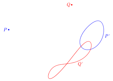
i) (2 points) Construct the circle along which the lens centre moves.
ii) (4 points) Determine the direction of the lens plane, i. e. construct a line parallel to the lens.
In the construction tasks, draw the construction on the provided sheet with the figure, detail the steps of your construction, and explain why your construction works.
Risposta: geometric construction — see the official solution
Soluzione:
i) (2 points) Let denote the circle traced by the lens centre. A light ray from that passes through the lens centre is undeflected, so it continues straight through to the image of at that instant. As moves around , the undeflected ray through and sweeps a family of lines through , and its intersection with the image curve gives the current image. The extreme angular positions of this sweep correspond to being at the tangent points of as seen from --- that is, the lines from that are tangent to . At these extreme instants the corresponding image point on is where the line from is tangent to the curve .
Hence: from , draw the two lines tangent to curve --- call them , with point and on curve . They are tangent to . Repeat from , drawing two lines tangent to --- call them with points and on curve . These are also tangent to . Four tangent lines determine the circle : for instance, the centre of lies at the intersection of the angle bisectors of any two pairs of these tangents (since each bisector is the locus of points equidistant from two lines). Project this centre perpendicularly onto any tangent to get the radius, and draw .
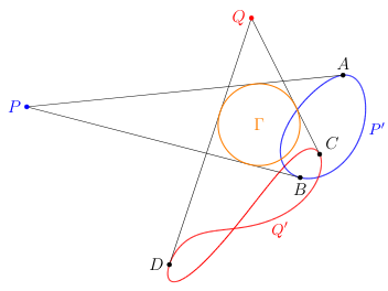
Grading:
-
Recognising that a ray from through the lens centre is undeflected 0.2 pts
-
Recognising that the tangents from to curve are tangent to 0.8 pts
-
Correct detailed construction idea of [from (at least three of) the four tangent lines] 0.5 pts
-
Correctly performed construction (i.e. constructed circle on paper is close to the actual circle) 0.5 pts
-
Only given if the construction corresponds to a correct idea
-
It is important that the circle intersects and not
-
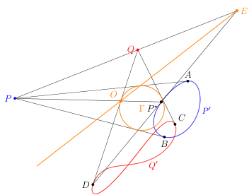
ii) (4 points) Fix any point on . It is enough to find one other point on the lens to draw the lens plane at this position. For this, we aim to identify the images of and for this chosen point for the centre of the lens.
Draw the line through and ; it extends to intersect curve possibly at two points. The intersection corresponding to the location of the lens needs to be determined. Using continuity and the reality of images: as moves continuously around , the image moves continuously on , and the tangent-correspondence from (i) matches regions of with regions of . (Moreover, near an intersection of with , the corresponding must be the far intersection of line with --- the near intersection would place the object within the focal region, making the image virtual.) This resolves the ambiguity and identifies as the current image of . For , the above identification procedure doesn’t work as it does not intersect and thus intersection with the focal region (a priori we do not know the focal length) is not guaranteed. Therefore, it is convenient to pick point to be such that is tangent to in which case there is only one valid point ( or ). In the figure, is chosen such that is , then is the closer intersection of with .
Now we have: object imaged to , object imaged to , through a lens with centre at . With two objects and their real images under a converging lens, the lens can be reconstructed. Suppose a light ray starts from toward . Then, as and are the images of and (and the lens is ideal), the ray must refract from the lens to form the line . Therefore the lines and intersect at the lens plane plane, identifying another point of the lens plane . Thus is the lens plane at the moment of time when the centre of the lens is at and is thus parallel to the lens plane at all moments in time.
Grading:
-
Idea: selecting a specific and intending to find its image pair to locate the lens plane 0.5 pts
-
Correct argument that the image points and object points are enough to find the lens plane (eg. analysing as a ray that refracts to a line through the image points) 0.5 pts
-
Justification for the correspondence between regions of and an image curve ( or ) 1 pts
-
Uses continuity of motion (to split image curve into regions corresponding to regions in ) 0.5 pts
- Given only if it is explicitly mentioned or implicitly used in correct reasoning to relate a point on to its unique real image in a non-trivial case
-
Uses correct reasoning to relate a point on to its unique real image 0.5 pts
-
-
Identifying the correct image point on (or , non-trivial case) 1 pts
- Correct point with no or weak justification 0.5 pts
-
Choosing point such that the image on (or ) is at the tangent (alternatively, a correct argument for finding the correct point on the other image curve (or )) 0.5 pts
- This point is given for finding the point on the other curve (in relation to items 3 and 4) with justification. Alternatively if student only has identified one point on one curve with just tangency, give 0.5 points for this and nothing for items 3 and 4.
-
Correctly performed construction (consistent with detailed steps to a correct construction) 0.5 pts
NB! Due to in accurately drawn diagrams, it can seem like that there is a lens position where will image to the intersection of and to one of its tangents . In this case identifying points and will in total give 2 points (instead of 1.5 points) which replaces items 3—5 in the above scheme. In addition 0.5 points will be given for an inaccurately drawn diagram. I.e. in this case maximum of points is 3.
Grading (replaces items 3—5)
-
Finding with two trivial points 2 pts
-
No points for correctly performed construction (due to inaccuracy)
Solution 2. This problem can also be solved using the lens formula. Namely, take the tangent lines (or if any two line for which you know how to identify the points). Take the angle between these lines and the angles and at which the optical axis (perpendicular to the lens) intersects these. From basic geometry (exact equation depends on the definitions). Now the lens positions and relevant, will split the lines in lengths and for one line and and for one line. Then the lens equation states (whether or not it is cosine or sine depends on the definitions). Now we have two equations and two unknowns. Thus (or ) can be solved and thus a parallel line drawn with a protractor.
Grading:
-
Image points identified correctly (either trivial or non-trivial with justification) 0.5
-
Lens formula written with respect to measured lengths (projected correctly) 0.5
-
Angle/direction solved correctly (all or nothing) 2.5
-
Correctly performed constructions (angles match) (only given for correctly calculated angle) 0.5
Official solution (NBPhO 2026, solutions v1.2 with grading scheme), from the official PDF; text as transcribed by olimpicos.net.
Topic: Geometric Optics Metodi: Ray Tracing, Thin Lens & Mirror Equation Competenze: Diagrammatic Reasoning Objects: Lens Fonte: Testo (PDF) — p.1 · Soluzione ufficiale (PDF)
Lente in movimento (6 punti) — Eppu Leinonen
Il centro di una lente sottile convergente si muove lungo una circonferenza, mentre l’orientazione della lente resta fissa; l’asse ottico della lente giace nel piano della circonferenza (il piano della figura). La lente forma le immagini di due punti fissi e , anch’essi in questo piano; le immagini sono sempre reali. Mentre la lente si muove, ciascuna immagine descrive una curva chiusa nel piano della figura: , . I due punti ed entrambe le curve sono mostrati in figura.
i) (2 punti) Costruisci la circonferenza lungo cui si muove il centro della lente.
ii) (4 punti) Determina la direzione del piano della lente, cioè costruisci una retta parallela alla lente.
Nei compiti di costruzione, traccia la costruzione sul foglio fornito con la figura, descrivi i passaggi e spiega perché la costruzione funziona.
Risposta: costruzione geometrica — vedi la soluzione ufficiale
Soluzione: La soluzione ufficiale completa (in inglese) è nella versione originale di questo quesito e nel PDF ufficiale.
Topic: Geometric Optics Metodi: Ray Tracing, Thin Lens & Mirror Equation Competenze: Diagrammatic Reasoning Objects: Lens Fonte: Testo (PDF) — p.1 · Soluzione ufficiale (PDF)
Lissajous bridge (6 points) — Jaan Kalda
A circuit has four nodes , , , . An AC source of amplitude is applied between and . A resistor connects to and a capacitor connects to ; a resistor connects to and an inductor connects to . A potentiometer with a sliding contact is connected between and . The voltage between and feeds the -input of an oscilloscope, and the voltage between and feeds the -input; both input channels have the same gain. The oscilloscope plots the voltage from the -input and the voltage from the -input in the —-plane. The position of the sliding contact is adjusted until the figure on the screen degenerates into a line segment. It appears that in that case, the line segment makes an angle with the -axis, and the sliding contact divides the potentiometer’s length in the ratio from left to right in the figure. Find the amplitude of the voltage between and .
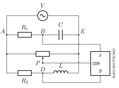
Risposta:
Soluzione:
Set and (phasor). Consider the RC branch: since and carry the same current, their voltages are in the impedance ratio . The factor is a clockwise rotation in the phasor plane, so is rotated clockwise --- in particular, , and lies in the lower half-plane ().
For the RL branch, : the factor is a counterclockwise rotation, so is rotated counterclockwise, giving and in the upper half-plane ().
By Thales’ theorem applied to each branch, both and lie on the circle of diameter (centre , radius ), on opposite semicircles.
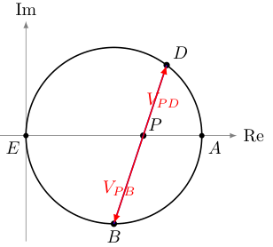
The oscilloscope displays on and on ; the Lissajous figure degenerates to a line when these phasors are parallel or antiparallel --- equivalently, when , , are collinear in the phasor plane. Since and are on opposite sides of the real axis, and is real (a fraction of ), lies between them on the line, so and are antiparallel. Hence the displayed line has negative slope and
The potentiometer is split 1:2 from left to right; depending on the orientation this gives or . The power of point with respect to the Thales circle,
takes the value in both cases (by symmetry of the quadratic about ). Since is inside the circle and the line cuts it at two points,
Combining with :
Grading: (6 points total)
-
Showing that 0.5 pts
-
Showing that 0.5 pts
-
Correctly identifying that lies in the lower half-plane () ( if ) 0.3 pts
-
Correctly identifying that lies in the upper half-plane () ( if ) 0.3 pts
-
Identifying that lies on a circle with as a chord 0.3 pts
-
Identifying that lies on a circle with as a chord 0.3 pts
-
Identifying as the diameter of the (common) circle 0.3 pts
-
Recognising that Lissajous degeneracy requires , , collinear in the phasor plane 1.5 pts
-
Applying power of a point at to get 1.0 pts
-
Correctly relating to the voltage amplitude ratio (only if phasors considered) 0.5 pts
-
Combining with the power-of-a-point result to obtain the final answer 0.5 pts
Since the condition the line segment makes an angle with the -axis could be understood in different ways, we did not deduct marks for failing to realize that the slope is negative or using without absolute value.
Alternative solution (pure algebraic/impedance method, for students who do not spot the Thales circle). Ground node and write . The voltage dividers at and give
and the resistive slider gives (or ; the answer is insensitive to this choice). Introduce dimensionless parameters and , so that
Taking , write and :
The Lissajous curve degenerates to a line iff is real, i.e., . Substituting and simplifying yields
so (since ) the bridge condition is , i.e., . The slope of the displayed line equals the ratio of the phasors (both now real), conveniently computed from imaginary parts:
Substituting gives
The amplitude between and follows from :
Using ():
Grading (alternative solution): 6 points total
-
Correctly computing as a phasor 0.5 pts
-
Correctly computing as a phasor 0.5 pts
-
Identifying (or ) 0.3 pts
-
Expressing and in the form with explicit real and imaginary parts 0.5 pts
-
Recognising that the Lissajous curve degenerates to a line iff is real (i.e., , or equivalent condition) 0.7 pts
-
Correctly deriving the bridge condition (equivalently ) 0.5 pts
-
Expressing in terms of and (or equivalent parameters) 0.5 pts
-
Substituting the bridge condition to write as a function of alone 0.5 pts
-
Correctly computing in terms of (before factoring) 0.7 pts
-
Recognising the factoring that simplifies 0.8 pts
-
Eliminating using the expression 0.3 pts
-
Obtaining the final answer 0.2 pts
Students who reach the correct final form via either route receive full credit. Algebraic errors may lose the corresponding stage points but could retain partial credit if the overall structure is right.
Official solution (NBPhO 2026, solutions v1.2 with grading scheme), from the official PDF; text as transcribed by olimpicos.net.
Topic: Circuits Metodi: Kirchhoff’s Laws, Vector Decomposition Competenze: Mathematical Modeling Objects: Resistor, Capacitor, Inductor Fonte: Testo (PDF) — p.1 · Soluzione ufficiale (PDF)
Ponte di Lissajous (6 punti) — Jaan Kalda
Un circuito ha quattro nodi , , , . Tra ed è applicato un generatore alternato di ampiezza . Un resistore collega a e un condensatore collega a ; un resistore collega a e un induttore collega a . Tra ed è collegato un potenziometro con contatto strisciante . La tensione tra e alimenta l’ingresso di un oscilloscopio e la tensione tra e l’ingresso ; i due canali hanno lo stesso guadagno. L’oscilloscopio traccia la tensione dell’ingresso e la tensione dell’ingresso nel piano –. La posizione del contatto viene regolata finché la figura sullo schermo degenera in un segmento. Si osserva che in tal caso il segmento forma un angolo con l’asse e che il contatto divide la lunghezza del potenziometro nel rapporto da sinistra a destra nella figura. Trova l’ampiezza della tensione tra e .
Risposta:
Soluzione: La soluzione ufficiale completa (in inglese) è nella versione originale di questo quesito e nel PDF ufficiale.
Topic: Circuits Metodi: Kirchhoff’s Laws, Vector Decomposition Competenze: Mathematical Modeling Objects: Resistor, Capacitor, Inductor Fonte: Testo (PDF) — p.1 · Soluzione ufficiale (PDF)
Kirill on a swing (8 points) — Kaarel Hänni
A swing has rigid rods attaching it to a horizontal pivot, so it can rotate freely in a vertical plane. Initially the swing hangs vertically below the pivot with Kirill standing upright on the seat; his friend gives him an initial angular velocity about the pivot. Kirill is practising athletic swinging: whenever the swing momentarily has zero angular velocity, he quickly squats; whenever the rods are again vertical, he quickly stands up. Treat Kirill as a point mass at distance from the pivot when standing and when squatting (); squatting and standing are motions along the rods. Neglect friction, air resistance, and the mass of the swing. Gravitational acceleration is .
i) (1.5 points) Sketch, qualitatively, how Kirill’s angular speed depends on time during the first full period of the swing.
ii) (2 points) On the phase diagram (angular velocity vs. angle), sketch, qualitatively, the trajectory from the initial push until the swing first goes over the top. The total number of periods shown need not be correct.
iii) (4.5 points) Find how many times Kirill must stand up before the swing first goes over the top. Evaluate your answer for , , , and .
Risposta: iii) stand-ups ()
Soluzione:
i) (1.5 points) Starting at the bottom with , Kirill (standing, radius ) swings up; falls smoothly to at the turning point, after a quarter-period . At the turning point Kirill squats (radius , no effect on the plot since ). Swinging back while squatting, rises smoothly from to (see part c; ) after a quarter-period , which is longer than the first since . At the bottom Kirill stands up: jumps from to . The second half of the period repeats the pattern with new amplitudes , , .
The sketch should therefore show:
-
smooth arches during swinging, cusps at the bottom (jumps) and smoothness at turning points;
-
the “squatting” arches taking longer than the “standing” ones;
-
growth of successive peaks.
Part (i): Angular speed vs time, first full period.
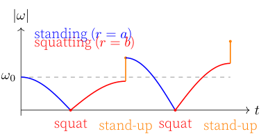
Part (i) --- qualitative sketch of (or signed ) vs :
-
Approximately sinusoidal arcs between jumps 0.3 pts
-
Instantaneous jumps at the maximum values of (at the bottom of the swing, during stand-up) 0.6 pts
-
Smaller amplitude during “squatting” arches, or equivalently a longer quarter-period while 0.3 pts
-
Overall growth of peak over the period 0.3 pts
A sketch of signed (rather than ) receives full credit if the curve correctly corresponds to the axis labels and all other qualitative features are preserved. Failure to correctly mark , where necessary, deducts 0.5 pts. The same goes for not completing the full period of the first swing.
ii) (2 points) The trajectory in the plane pieces together arcs of pendulum-like phase curves at two radii, and . Each half-swing traces an arc of the energy conservation curve for the relevant radius. Stand-ups at appear as vertical segments where jumps from to . Squats at the turning points () appear as smooth transitions (the radius- arc meets the radius- arc tangentially at ).
The motion is an outward spiral: each full cycle brings Kirill back to with a larger . When at the bottom (standing, radius ) first exceeds , the next upward arc does not close: it reaches with and continues past the top. This is the open curve on the sketch.
Part (ii): Phase diagram ( vs ), first three half-swings.
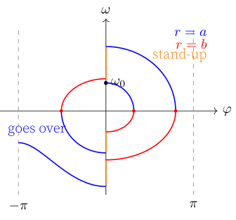
Key features for grading:
-
lens-shaped/pendulum-like arcs (not ellipses);
-
vertical line segments only at (stand-ups), smooth meeting at turning points (squats);
-
spiral grows outward;
-
final open curve goes over the top with non-zero .
Failure to use the phase diagram of angular velocity and angle, deducts 0.5 pts from the sum of part ii).
The number of spiral loops is not required to match the actual answer computed in part (c).
Part (ii) --- qualitative sketch of phase diagram vs :
-
Elliptical arcs for small-amplitude (early) cycles, with standing arcs () visibly taller (steeper in ) than squatting arcs () 0.5 pts
-
Trajectory passes continuously through the turning points (): no jump at maximum 0.3 pts
-
Vertical jumps at (during stand-up at the bottom): jumps by factor 0.4 pts
-
Overall growth: each successive cycle encloses the previous one, spiralling outward 0.4 pts
-
Final half-cycle goes over the top --- trajectory crosses with still nonzero (no turning point on this segment) 0.4 pts
iii) (4.5 points) Growth factor per stand-up. Let denote the angular velocity just after the -th stand-up (at the bottom, standing, radius ); let denote the angular velocity just before that stand-up (at the bottom, squatting, radius ).
Energy conservation on the way up (standing, radius ) to turning point at angle : At the turning point , so the squat () leaves and unchanged. Swinging back down (squatting, radius ): Equating: . The stand-up is a purely radial motion, so angular momentum about the pivot is conserved: , whence After stand-ups, .
Minimum angular velocity for a loop. The rods are rigid, so the condition for reaching the top is simply that the kinetic energy at the bottom suffice to raise Kirill by :
Counting. Kirill first loops over when , i.e.
Numerical evaluation. With , , , :
Check: rad/s (just short); rad/s (exceeds ). So Kirill loops over on the swing-up following his sixth stand-up.
Grading (part c):
-
Angular momentum conservation during the stand-up 0.7 pts
-
Energy conservation during the swing 0.7 pts
-
Growth factor per stand-up 0.7 pts
-
Minimum angular velocity for the rigid-rod swing to loop over the top 0.8 pts
-
Correct inequality for the over-the-top condition ( after the th stand-up) 0.4 pts
-
Solving the inequality for using the growth law , yielding 0.7 pts
-
Numerical answer 0.5 pts
Official solution (NBPhO 2026, solutions v1.2 with grading scheme), from the official PDF; text as transcribed by olimpicos.net.
Topic: Rotational Dynamics, Oscillations & Waves Metodi: Torque & Angular Momentum Analysis, Energy Conservation Method Competenze: Physical Reasoning, Diagrammatic Reasoning Objects: Pendulum, Rod Fonte: Testo (PDF) — p.1 · Soluzione ufficiale (PDF)
Kirill sull’altalena (8 punti) — Kaarel Hänni
Un’altalena è collegata a un perno orizzontale da aste rigide, così che può ruotare liberamente in un piano verticale. Inizialmente l’altalena pende verticalmente sotto il perno, con Kirill in piedi sul sedile; un amico gli imprime una velocità angolare iniziale attorno al perno. Kirill si allena a dondolarsi in modo atletico: ogni volta che l’altalena ha velocità angolare istantaneamente nulla si accovaccia rapidamente; ogni volta che le aste tornano verticali si rialza rapidamente. Tratta Kirill come una massa puntiforme a distanza dal perno quando è in piedi e quando è accovacciato (); accovacciarsi e rialzarsi sono movimenti lungo le aste. Trascura attriti, resistenza dell’aria e massa dell’altalena. L’accelerazione di gravità è .
i) (1,5 punti) Disegna qualitativamente come dipende dal tempo la velocità angolare di Kirill durante il primo periodo completo dell’altalena.
ii) (2 punti) Sul diagramma di fase (velocità angolare in funzione dell’angolo) disegna qualitativamente la traiettoria dalla spinta iniziale fino a quando l’altalena compie per la prima volta il giro completo. Il numero totale di periodi rappresentati non deve essere necessariamente corretto.
iii) (4,5 punti) Trova quante volte Kirill deve rialzarsi prima che l’altalena compia per la prima volta il giro completo. Calcola il risultato per , , e .
Risposta: iii) volte ()
Soluzione: La soluzione ufficiale completa (in inglese) è nella versione originale di questo quesito e nel PDF ufficiale.
Topic: Rotational Dynamics, Oscillations & Waves Metodi: Torque & Angular Momentum Analysis, Energy Conservation Method Competenze: Physical Reasoning, Diagrammatic Reasoning Objects: Pendulum, Rod Fonte: Testo (PDF) — p.1 · Soluzione ufficiale (PDF)
Rod and bead (8 points) — Eero Ristolainen, Jaan Kalda
A bead is threaded on a rigid frictionless rod. The rod rotates with constant angular velocity about a horizontal axis that is perpendicular to the rod and passes through a fixed point on it. Gravitational acceleration is .
i) (1 point) With suitable initial conditions, the trajectory of the bead is a circle. Sketch this trajectory in the plane perpendicular to the rotation axis, in a coordinate system with the axis at the origin.
ii) (1 point) Given that the trajectory is exactly a circle, find its radius.
iii) (2 points) The circular trajectory of the previous tasks is unstable. To stabilise it, one attaches a spring that produces a restoring force when the bead is displaced by along the rod from the axis of rotation. For what values of the stiffness can the bead move along a stable circular trajectory, and what is the radius of such a trajectory?
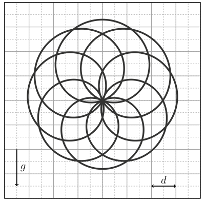
iv) (4 points) Next, the spring is removed, the bead is given a charge , and a uniform electric field of strength whose vector rotates with angular velocity in the same direction as the rod is introduced. With suitable initial conditions, the bead follows the trajectory shown below. Find , , and the ratio , where is the mass of the bead, in terms of and , the side length of the grid squares shown in the figure. You may take measurements from the figure.
Risposta: ii) ; iii) , ; iv) , ,
Soluzione:
i) (1 point) Solution 1 by Eero Ristolainen: The bead must pass through the origin (rotation axis). Otherwise, the bead would stay on “one side of the rod” and thus at the lowest point of the trajectory the force exerted by the rod couldn’t be entirely vertical and thus it couldn’t be the lowest point. Hence, the bead must pass through the origin at the lowest point of the trajectory which corresponds to the rod being horizontal. This is enough to make a sketch: the path is a circle of radius centred at .
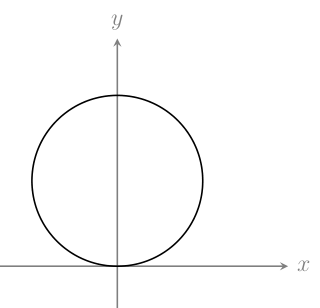
Solution 2: The plot can be made also from solution 4 of part ii.
-
Correct sketch 1 pts
- Otherwise correct sketch without axis 0.5 pts.
ii) (1 point)
Solution 1 by Eppu Leinonen: The bead’s velocity normal to the rod has to be the same as the rod’s velocity at that point for the bead to stay on the rod. At the topmost point the bead has no radial velocity. Thus, at the topmost point . On the other hand, at the topmost point (from Newton’s law) and from centripetal acceleration we can solve .
Solution 2 by Eero Ristolainen, Eppu Leinonen: The circular motion must be uniform as the rod performs uniform circular motion. A straight forward formal proof for the this follows from the inscribed angle theorem. The angle of the bead measured from the centre of the rod is twice the angle measured from the origin at the circumference of the circle. The latter changes with speed as the corresponding straight line is the rod, thus the former must be . Thus the centripetal acceleration on the bead is . At the topmost point, the speed is and the acceleration is only due to gravity and is . Thus .
Grading (solutions 1 and 2 or similar):
-
Recognises that the normal velocity of the bead to the rod is the rod’s velocity (implicitly or explicitly) OR a valid argument for uniform circular motion with 0.2 pts
-
at the topmost point 0.2 pts
-
At the topmost point 0.2 pts
-
0.2 pts
-
Correct answer 0.2 pts
Solution 3 by Eero Ristolainen: The centre of the motion is and the angular velocity is since the bead performs a circle on both sides of the rod. Thus the coordinates of the bead with respect to time are where is the location of the bead measured from the axis of rotation (and taking into account the direction). In the frame of the rod, the equation of motion is since Coriolis force is perpendicular to the direction of motion which is counteracted by the rod. Substituting the above expression yields the answer.
Grading:
-
A valid argument for uniform circular motion with 0.2 pts
-
Parametrisation of the circle with respect to angle () and 0.2 pts
-
Correct equation of motion in the rotating frame 0.2 pts
-
Explains why Coriolis force doesn’t matter 0.2 pts
-
Correct answer 0.2 pts
Solution 4 by Eppu Leinonen, Eero Ristolainen: Go to the corotating frame of the rod. Since the bead is moving in this rotating frame, it experiences a Coriolis force. However, it is directed perpendicular to the velocity which is limited to be along the rod. Hence, it does not affect the equation of motion of the bead and can be ignored. Let be the coordinate of the bead along the rod (with sign determining the direction). Then the equation of motion along the rod is This gives an inhomogeneous second order linear differential equation The general solution is a sum of the general solution to the homogenous problem and any solution to the inhomogeneous problem. The homogenous solution is A particular solution we can guess by substituting . This gives an equation for as and thus . Thus the general solution is which can only be periodic (in finite time) if , which determines the initial conditions (which of there are only one) for the bead to have a circular trajectory. In the lab frame: This is a circle of radius centred at (which gives the solution to part i as well).
Grading:
-
Correct equation of motion in the rotating frame 0.2 pts
-
States implicitly or explicitly that the general solution to the differential equation is the sum of the homogeneous and particular solutions 0.2 pts
-
Correct homogenous solution 0.1 pts
-
Correct particular solution 0.2 pts
-
States that homogenous solution corresponding to periodic motion is 0 0.1 pts
-
Correct answer 0.2 pts
iii) (2 points) Solution 1 by Jaan Kalda, Eero Ristolainen, Eppu Leinonen With the spring, the equation of motion becomes
Stability. Perturbations from the periodic particular solution obey the homogeneous equation . If (i.e., ), this is simple harmonic motion at frequency --- perturbations remain bounded, orbit is stable. If , perturbations grow exponentially --- unstable. The stability criterion is The centrifugal term acts as an effective destabilising stiffness , and the spring must overcome it.
As in solution 2 to part ii, we again look at the topmost point of the trajectory. The velocity is again , but now the acceleration is . Solving this gives . In the case the radius becomes negative, the circular trajectory simply appears below the origin, so we can take the magnitude of the radius above, giving the final result:
Grading:
-
Equation of motion including the spring 0.2 pts
-
Idea of looking at (small) displacements to analyse stability 0.3 pts
-
Identifying the homogeneous equation governing perturbations 0.5 pts
-
Correct stability criterion 0.3 pts
-
Correct equations for the acceleration and velocity at the top of the trajectory 0.5 pts
-
Correct radius formula 0.2 pts
Solution 2 by Jaan Kalda (for finding the radius) The particular solution is again (as in solution 4 to part ii) :
The corresponding lab-frame orbit is, as in (b), a circle of radius , giving the result as in solution 1. For the amplitude is positive and the circle sits above the axis (as in parts a, b); at the driven amplitude diverges (driving resonance --- the bounded circular orbit ceases to exist); for the amplitude is negative, meaning the circle flips to below the axis, but remains stable. Grading:
-
Solving for particular-solution amplitude 0.5 pts
-
Correct radius formula 0.2 pts
Solution 2 by Eppu Leinonen Alternatively following solution 4 of part ii, the general solution to this differential equation can be found. However, now the homogenous solution is sum of real exponentials if which is unstable and a sum of sinusoid if which is stable. Then the particular solution can be guessed the same way as in the solution above.
iv) (4 points) Solution by Eero Ristolainen and Eppu Leinonen
Now the equation of motion in the frame of the rod is: Let us write as the angular velocity of the electric field in the frame of the rod. From the figure we see that is a sum of two periodic components . Furthermore, the linearity of the differential equation gives us that The first one is fulfilled by the exact same solution as before (deduced the same way as in solution 2 of part), . We guess the second solution to be of the form , which gives .
We see that the solution is periodic. Let this period be . Then we must have that with some positive integers and where and are the periods of and respectively. We notice that the figure is almost symmetric with respect to -axis, which is a huge deviation from the solution with just . Thus the amplitude of must dominate the one of . Therefore, the sign changes changes of corresponds to the loops in the figure which there are 8 of. Since the sine function has changes sign twice in a period, we get .
For the motion to reach the same ray (from origin, an example dashed in the figure below) twice, it takes time (the rod has made half a turn). From the graph, we can read that in time (red + blue) the bead travels less distance than in (red+blue+orange). Similarly in time (red + blue + orange + the rest of the black to the horizontal axis) the bead travels more than in (red + blue + orange).
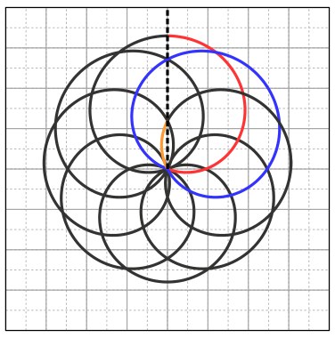
Thus we get the following inequalities which gives for which is the only solution. I.e. we get (This can also be recovered from there being 4 loops corresponding to 5 -intercepts corresponding to the rod being vertical. This automatically gives .)
The symmetry with respect to reflection along the -axis in the figure (the trajectory is parallel to the -axis at the extremal points on the -axis) dictates that the electric field must point vertically when the bead is on the extremal points on the -axis. Thus, the corresponding displacements along these extremal -points must align constructively or destructively. I.e. the top-most and bottom-most distances from the origin correspond to the cases (The formal justification is that at these extremal points and both contributions are proportional to a sinusoid, thus and are “orthogonal” at the same points. Thus, as gravity is parallel to the rod we have is at its extremum and thus . Thus and thus contribution from has to be at its extremum. This implies that the electric field points parallel or anti parallel to the rod at these extremal points. Now (due to both being orthogonal to ) and thus at these extremal points on the -axis, we have and .)
Measuring and solving gives
Grading:
-
Equation of motion including the electric field 0.1 pts
-
Writing 0.1 pts
-
Deducing 0.2 pts
-
Guessing 0.2 pts
-
Finding 0.2 pts
-
Realising dominates with proper reasoning 0.5 pts
-
Noting periodicity 0.2 pts
-
0.2 pts
-
Finding a restrictive enough inequality for (or ) from the figure (or any other procedure that works for finding ) 0.8 pts
- For a correct idea (in case it is executed wrong) 0.2 pts
-
0.1 pts
-
0.2 pts
-
Deducing with reasonable explanation that electric field points along the -axis when bead reaches extremal 0.5 pts
-
Writing and as the difference/sum of the and amplitudes 0.3 pts
-
Solving for and 0.1 pts
-
and 0.3 pts
-
0.1pt for one correct.
-
,
-
Official solution (NBPhO 2026, solutions v1.2 with grading scheme), from the official PDF; text as transcribed by olimpicos.net.
Topic: Newtonian Mechanics, Electrostatics Metodi: Differential Equations, Superposition Principle Competenze: Mathematical Modeling, Diagrammatic Reasoning Objects: Rod, Ball, Spring Fonte: Testo (PDF) — p.1 · Soluzione ufficiale (PDF)
Asta e perlina (8 punti) — Eero Ristolainen, Jaan Kalda
Una perlina è infilata su un’asta rigida senza attrito. L’asta ruota con velocità angolare costante attorno a un asse orizzontale perpendicolare all’asta e passante per un suo punto fisso. L’accelerazione di gravità è .
i) (1 punto) Con opportune condizioni iniziali la traiettoria della perlina è una circonferenza. Disegna questa traiettoria nel piano perpendicolare all’asse di rotazione, in un sistema di coordinate con l’asse nell’origine.
ii) (1 punto) Sapendo che la traiettoria è esattamente una circonferenza, trova il suo raggio.
iii) (2 punti) La traiettoria circolare delle domande precedenti è instabile. Per stabilizzarla si aggiunge una molla che esercita una forza di richiamo quando la perlina è spostata di lungo l’asta rispetto all’asse di rotazione. Per quali valori della costante elastica la perlina può muoversi lungo una traiettoria circolare stabile, e qual è il raggio di tale traiettoria?
iv) (4 punti) Si toglie poi la molla, si dà alla perlina una carica e si introduce un campo elettrico uniforme di intensità il cui vettore ruota con velocità angolare nello stesso verso dell’asta. Con opportune condizioni iniziali la perlina segue la traiettoria mostrata qui sotto. Trova , e il rapporto , dove è la massa della perlina, in funzione di e di , lato dei quadretti della griglia in figura. Puoi prendere misure dalla figura.
Risposta: ii) ; iii) , ; iv) , ,
Soluzione: La soluzione ufficiale completa (in inglese) è nella versione originale di questo quesito e nel PDF ufficiale.
Topic: Newtonian Mechanics, Electrostatics Metodi: Differential Equations, Superposition Principle Competenze: Mathematical Modeling, Diagrammatic Reasoning Objects: Rod, Ball, Spring Fonte: Testo (PDF) — p.1 · Soluzione ufficiale (PDF)
Saturation pressure of water (8 points) — Eero Uustalu
Experimental problem. Tools: transparent plastic tube (open at both ends, Luer lock to connect with a syringe at one end, length , inner diameter ); plastic syringe with a water-tight Luer fitting to the tube; small open container with a few millilitres of dodecane (labelled “D”); metal pin with outer diameter to close the tube tightly (if it gets stuck, ask the invigilator to help remove it); measuring tape; container with water (labelled “W”); a large container for waste liquids; a small wooden stick; a few strips of masking tape; paper towel.
Water and dodecane do not dissolve in each other. The density of dodecane is less than the density of water.
Avoid skin and eye contact with dodecane, and do not ingest it; wash your hands after handling.
During the experiment, the tube can only be filled with dodecane: the inner surface of the tube must never touch water!
If necessary, you can have one replacement tube, one replacement syringe, and reasonable additional amounts of dodecane and water.
Determine the saturated vapour pressure of water at room temperature; room temperature and air pressure are recorded by the invigilator at the start of the session: ; .
Note that at typical room temperatures, the saturated vapour pressure of dodecane is much lower than that of water.
i) (2 points) Describe your measurement procedure and explain the physical principle it is based on.
ii) (4 points) Perform the measurements. Tabulate all quantities you measure and document the sequence of operations.
iii) (2 points) Determine at room temperature. What is the dominant source of systematic error?
Risposta: experimental — e.g. at (see the official solution)
Soluzione:
Main idea. Use a sealed air bubble as a manometer. If we can trap a small air bubble somewhere in the tube, note its initial length under atmospheric pressure, and then reduce the pressure in the bubble, the bubble’s length grows. Since the tube’s cross-section is uniform, the bubble’s pressure is determined by the ideal gas law (isothermal expansion):
If we reduce the air bubble’s pressure by pulling on the syringe plunger, dodecane carries the reduced pressure from the air bubble back through the tube to the water—dodecane interface inside the syringe. Once the pressure there drops to , water vapour starts forming bubbles at the interface, which grow and coalesce. At that point, pulling the syringe further no longer reduces the air bubble’s pressure: any further pressure drop is immediately compensated by additional vapour evaporating at the interface. So once the air bubble stops growing in response to syringe pulling, we have (plus a small hydrostatic correction if the tube is not laid horizontally; see below).
Why dodecane? The role of dodecane is to act as an incompressible, non-volatile piston between the syringe and the air bubble. Dodecane is hydrophobic, does not dissolve in water, and has negligible vapour pressure at room temperature (as stated in the problem). It is also lighter than water, so water stays below dodecane in any at-rest configuration.
The problem warns that water must not touch the inner surface of the tube, because traces of water get adsorbed onto the plastic wall. When the pressure in the tube is then reduced below , these adsorbed traces boil off, forming a series of small bubbles distributed along the tube. Each such bubble also expands during the measurement, adding uncontrolled volume to the gas column and distorting the -to- ratio. By filling the tube with dodecane before introducing any water, the inner surface is prewetted with a hydrophobic liquid that excludes water from the wall.
Design. The tube must contain dodecane filling it from the syringe end up to a small air bubble of initial length at the far end (closed by the metal pin). Water sits in the syringe itself, not in the tube. The air bubble cannot be too small (initial length reading becomes imprecise) nor too large: during the measurement it expands by a factor of (since at room temperature), so an initial bubble of expands to , comfortably fitting in a tube. Any additional air bubbles elsewhere in the tube or in the syringe would also expand during the measurement, distorting the result or making it impossible to reach within the full travel of the syringe plunger.
Note on orientation: the dodecane column has density , so a vertical column of dodecane produces a hydrostatic pressure difference of --- several times larger than the being measured. The tube must therefore be laid horizontally, otherwise the hydrostatic correction will dominate the result.
Preparation.
-
Connect the syringe to the tube.
-
Dip the far end of the tube into the dodecane container and pull the syringe plunger; dodecane fills the tube.
-
Lift the far end of the tube out of the dodecane and pull in a small amount of air, forming an air bubble of initial length at the far end.
-
Close the far end of the tube tightly with the metal pin.
-
Disconnect the syringe (keeping the plunger in place so no air enters the syringe from the open end).
-
Pull a small amount of water () into the syringe.
-
Reconnect the syringe to the tube (a small air bubble at the Luer joint is tolerable, but minimise it).
At this point, from syringe end to far end: syringe (with water) --- water—dodecane interface near the Luer joint --- dodecane filling the tube --- air bubble at the far end --- metal pin closure.
Measurement.
-
Lay the tube horizontally to avoid any hydrostatic correction in the dodecane column.
-
Measure the initial bubble length . Record the atmospheric pressure and the room temperature from the invigilator.
-
Pull the syringe plunger slowly. The bubble grows as the pressure drops. Continue until the bubble stops growing (the limit where ). Fix the plunger at this position.
-
Measure the final bubble length .
Typical values: , to (depending on room temperature; at , gives , so ).
Calculation. From the ideal gas law at constant temperature, With , , :
Dominant source of systematic error. Incomplete saturation: it takes time for water to evaporate at the interface inside the syringe, and if the plunger is pulled too fast, the pressure temporarily falls below (supersaturated vapour). The measured is then larger than its true equilibrium value, giving an underestimate of . Mitigation: pull slowly and wait for the bubble to stabilise before recording .
A secondary source is residual air: from the Luer joint, from air dissolved in the dodecane, or from water traces adsorbed on the tube wall (if dodecane pre-wetting was imperfect). These behave as additional gas in the air bubble and artificially reduce the apparent . Careful preparation --- filling the tube with dodecane before any water enters, keeping the water—dodecane interface inside the syringe, and avoiding air at the Luer joint --- minimises this.
Grading for methods similar to official solution, that don’t need to know the partial water pressure of the ambient room air. (8 points total)
For methods that require knowing the partial water pressure of the ambient room air, look at alternate scheme.
Part (i) --- description of procedure and principle (2 points).
-
Main idea: using the air bubble as a manometer 0.5 pts
-
Recognising that when the bubble stops growing under syringe pulling 0.5 pts
-
Correct role of dodecane: serves as piston; negligible vapour pressure; prevents water from wetting tube walls 0.6 pts
-
Application of the ideal gas law (or equivalent isothermal pressure—volume relation) to relate initial and final bubble lengths to pressures 0.4 pts
Part (ii) --- performing the measurements (4 points).
-
Correct tube preparation: dodecane fills the entire tube, small air bubble at the far end, water in the syringe 1.0 pts
-
Correct choice of initial bubble length (approximately to ) 0.5 pts
-
Documentation of preparation steps with a clear sequence 0.5 pts
-
Tabulation of the measured quantities and 0.8 pts
-
Recording atmospheric pressure and room temperature 0.2 pts
-
Slow pulling of the syringe / waiting for stabilisation 0.6 pts
-
Tube laid horizontally (or a correction applied if vertical) 0.4 pts
Part (iii) --- determination of and systematic error (2 points).
-
Correct computation of from , , 0.4 pts
-
Result within a factor of 1.5 of the expected value for the measured 1.2 pts
-
Otherwise, within a factor of 2 of the expected value 0.6 pts
-
Otherwise, within a factor of 3 of the expected value 0.3 pts
-
Identification of incomplete saturation (or a comparable dominant systematic source) 0.4 pts
(The three tolerance bands are mutually exclusive: award only the highest band the result falls in.)
Grading (methods that depend on knowing the partial pressure of ambient water moisture in the room air). (Maximally 5.6 points of 8 points total.)
The summary of these solutions is that they had a “dry” end of the long tube, with some dodecane in the middle to act as a piston, and the other end of the tube having the syringe on it, with some water in it. Over enough time, the water in the syringe will evaporate (raising the partial pressure of water, from the room’s ambient water vapor pressure, to the saturated vapor pressure), moving the dodecane piston towards the dry end.
If the dry end of the long tube was sealed, additional assumptions have to be made, which have to be explicitly justified.
Part (i) --- description of procedure and principle (2 points).
-
Explicitly stating, that the result comes to be lower than the real saturated vapor pressure of water, due to the ambient room air (and as such, the near end of the syringe where the water evaporates) also having water vapor already in it 1.6 pts
-
Application of the ideal gas law 0.4 pts
Part (ii) --- performing the measurements and calculating the expressions (max 3.2 out of 4 points).
For the sake of clarity, let’s say that the room air pressure is , length from the end of the dodecane until the (dry) end of the tube is , and the volume of the entire half of the system from the dodecane of the syringe side to be . Likewise, the respective new pressure, length, and volume, after the water vapor pressure has reached saturation on the syringe side, to be , , and .
-
Expressing if the dry end is sealed (or if dry end is left open) 1 pts
-
If it’s explicitly stated how/why , due to or something similar. (give automatically if dry end was left unsealed) 1 pts
-
Documentation of preparation steps with a clear sequence 0.3 pts
-
Recording atmospheric pressure and room temperature 0.2 pts
-
Waiting for stabilisation 0.3 pts
-
Tube laid horizontally (or a correction applied if vertical) 0.4 pts
Part (iii) --- determination of systematic error, sourcing from other than that of the ambient room’s water vapor pressure (max 0.4 points out of 2 points).
- Identification of incomplete saturation (or a comparable dominant systematic source) 0.4 pts
Official solution (NBPhO 2026, solutions v1.2 with grading scheme), from the official PDF; text as transcribed by olimpicos.net.
Topic: Thermodynamics, Fluid Mechanics Metodi: Hydrostatic Equilibrium, Ideal Gas Law, Experimental Data Analysis Competenze: Measurement & Instrumentation, Experimental Data Analysis Objects: Tube, Gas Fonte: Testo (PDF) — p.1 · Soluzione ufficiale (PDF)
Tensione di vapore saturo dell’acqua (8 punti) — Eero Uustalu
Problema sperimentale. Materiale: tubo di plastica trasparente (aperto alle due estremità, con attacco Luer a un’estremità per collegare una siringa, lunghezza , diametro interno ); siringa di plastica con raccordo Luer a tenuta d’acqua per il tubo; piccolo contenitore aperto con alcuni millilitri di dodecano (etichetta “D”); spillo metallico di diametro esterno per chiudere ermeticamente il tubo (se si incastra, chiedi aiuto al sorvegliante per toglierlo); metro a nastro; contenitore con acqua (etichetta “W”); un grande contenitore per i liquidi di scarto; un bastoncino di legno; alcune strisce di nastro adesivo di carta; carta assorbente.
Acqua e dodecano non si mescolano. La densità del dodecano è minore di quella dell’acqua.
Evita il contatto del dodecano con pelle e occhi e non ingerirlo; lavati le mani dopo averlo maneggiato.
Durante l’esperimento il tubo può essere riempito solo di dodecano: la superficie interna del tubo non deve mai toccare l’acqua!
Se necessario puoi avere un tubo e una siringa di ricambio e quantità aggiuntive ragionevoli di dodecano e acqua.
Determina la tensione di vapore saturo dell’acqua a temperatura ambiente; temperatura ambiente e pressione dell’aria vengono annotate dal sorvegliante all’inizio della sessione: ; .
A temperatura ambiente la tensione di vapore saturo del dodecano è molto minore di quella dell’acqua.
i) (2 punti) Descrivi la procedura di misura e spiega il principio fisico su cui si basa.
ii) (4 punti) Esegui le misure. Riporta in tabella tutte le grandezze misurate e documenta la sequenza delle operazioni.
iii) (2 punti) Determina a temperatura ambiente. Qual è la principale fonte di errore sistematico?
Risposta: sperimentale — ad es. a (vedi la soluzione ufficiale)
Soluzione: La soluzione ufficiale completa (in inglese) è nella versione originale di questo quesito e nel PDF ufficiale.
Topic: Thermodynamics, Fluid Mechanics Metodi: Hydrostatic Equilibrium, Ideal Gas Law, Experimental Data Analysis Competenze: Measurement & Instrumentation, Experimental Data Analysis Objects: Tube, Gas Fonte: Testo (PDF) — p.1 · Soluzione ufficiale (PDF)
Pull-up bar rope (5 points) — Jaan Kalda
A rope is thrown over a horizontal pull-up bar at height above the frictionless floor. One end of the rope is tied to a heavy weight resting on the floor; the other end is pulled so that the length of the rope between the bar and the weight decreases at a constant rate . At a given moment, this segment makes an angle with the vertical (see figure); the weight is still in contact with the floor. Gravitational acceleration is .
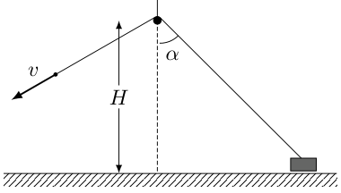
i) (1 point) Find the speed of the weight.
ii) (1 point) Find the magnitude of the acceleration of the weight.
iii) (3 points) Find the angle at which the weight lifts off the floor.
Risposta: i) ; ii) ; iii)
Soluzione:
i) (1 point) Place the bar at the origin of a coordinate system where is the horizontal distance from the bar to the weight along the floor, and is the height of the bar above the floor. The length of the bar-to-weight rope segment is
Method 1 (inextensibility / velocity projection). Since the rope is inextensible, the velocity components of its two endpoints along the rope direction must match: whatever rate one end recedes from a point on the rope, the other end must approach it at the same rate. The puller’s hand pulls the rope along its own direction at speed , so the rope shortens at rate . The weight moves horizontally toward the bar at speed ; its velocity component along the rope (which makes angle with the vertical, hence angle with the floor) is . Equating:
Method 2 (implicit differentiation). Differentiating with respect to time: With (the segment shortens at constant rate) and :
Grading (Method 1).
-
Recognising that the velocity components of the rope endpoints along the rope direction must match (rope inextensibility) 0.4 pts
-
Identifying the projection for the weight’s velocity along the rope 0.3 pts
-
Final answer 0.3 pts
Grading (Method 2).
-
Setting up with 0.3 pts
-
Correctly differentiating to obtain 0.4 pts
-
Final answer 0.3 pts
ii) (1 point) Method 1 (continuing from ). Differentiate again, with constant (so ): Since , we have : the weight accelerates toward the bar. With and :
- Correctly differentiating an incorrect result from the previous part 0.5 pts.
Method 2 (direct differentiation of ). The angle changes in time as the weight slides; introduce (positive as decreases). The weight’s position is , so its speed is Combined with : Differentiating with respect to time: Substituting :
Grading (Method 1).
-
Differentiating to obtain 0.5 pts
-
Substituting and to obtain final answer 0.5 pts
Grading (Method 2).
-
Introducing as the angular rate of the rope direction 0.2 pts
-
Relating the weight’s speed to : 0.2 pts
-
Deriving from 0.2 pts
-
Differentiating to obtain 0.2 pts
-
Substituting and obtaining final answer 0.2 pts
iii) (3 points) While the weight is on the floor, the only horizontal force on it is the horizontal component of the rope tension , directed toward the bar. Newton’s second law in the horizontal direction: Vertically, , where is the normal force from the floor. The weight lifts off when , i.e., :
Grading.
-
Identifying that the only horizontal force on the weight is 0.3 pts
-
Writing Newton’s second law horizontally: 0.3 pts
-
Substituting the expression for from part (ii) 0.2 pts
-
Isolating to obtain 0.2 pts
-
Correctly setting up the vertical force balance 0.5 pts
-
Correct lift-off condition , i.e., 0.5 pts
-
Algebraic manipulation to 0.5 pts
-
Final answer 0.5 pts
Official solution (NBPhO 2026, solutions v1.2 with grading scheme), from the official PDF; text as transcribed by olimpicos.net.
Topic: Newtonian Mechanics Metodi: Kinematic Equations, Free-Body Diagram Competenze: Mathematical Modeling Objects: String, Block Fonte: Testo (PDF) — p.2 · Soluzione ufficiale (PDF)
La fune sulla sbarra (5 punti) — Jaan Kalda
Una fune è gettata sopra una sbarra orizzontale per trazioni, posta ad altezza sopra un pavimento senza attrito. Un’estremità della fune è legata a un peso pesante appoggiato sul pavimento; l’altra viene tirata in modo che la lunghezza del tratto di fune tra la sbarra e il peso diminuisca a ritmo costante . In un certo istante questo tratto forma un angolo con la verticale (vedi figura); il peso è ancora a contatto con il pavimento. L’accelerazione di gravità è .
i) (1 punto) Trova la velocità del peso.
ii) (1 punto) Trova il modulo dell’accelerazione del peso.
iii) (3 punti) Trova l’angolo al quale il peso si stacca dal pavimento.
Risposta: i) ; ii) ; iii)
Soluzione: La soluzione ufficiale completa (in inglese) è nella versione originale di questo quesito e nel PDF ufficiale.
Topic: Newtonian Mechanics Metodi: Kinematic Equations, Free-Body Diagram Competenze: Mathematical Modeling Objects: String, Block Fonte: Testo (PDF) — p.2 · Soluzione ufficiale (PDF)
Water hose (5 points) — Ralf Robert Paabo
A liquid with density flows in a pipe with diameter . At low mean speeds , the flow is laminar (uniform and without vortices); the drag force per unit area on the liquid comes from wall friction, where (unit ) is the dynamic viscosity, is the local speed, and is the distance from the axis. When is large enough, the flow becomes turbulent, filled with vortices whose velocity fluctuations are of the order of itself. The drag still comes from wall friction , but the vortices squeeze the near-wall layer (across which the flow speed drops from to zero) to a thickness where the drag force per unit area is of the order of the dynamic pressure carried by the vortices.
i) (1.5 points) At any given flow speed, only one of the two mechanisms actually dominates the drag – but the dimensionless ratio of the two characteristic drag scales, , can be computed regardless and tells us which regime we are in. This ratio is the Reynolds number. Express as a product of powers of , , , and .
A water pump with output power is used for watering a garden; it draws water from a depth directly into a hose of length and inner diameter . Water leaves the end of the hose at a volumetric rate . Density of water is , viscosity and gravitational acceleration is .
ii) (0.5 points) Determine the flow type in the hose. It is known that flow is turbulent when and laminar otherwise.
iii) (3 points) The gardener is cleaning tools by directing the water jet onto dirty surfaces. Where the jet meets the surface, the pressure rises above atmospheric; this excess pressure is what removes dirt. To make cleaning more efficient, the gardener attaches a spray nozzle set to narrow-jet mode, so that the exit cross-section of the nozzle is of the hose’s cross-section. By what factor does the volumetric flow rate change? By what factor does the excess pressure at the dirty surface change? Find both within accuracy. You are allowed to use numerical methods.
Risposta: i) ; ii) turbulent; iii) , excess pressure
Soluzione:
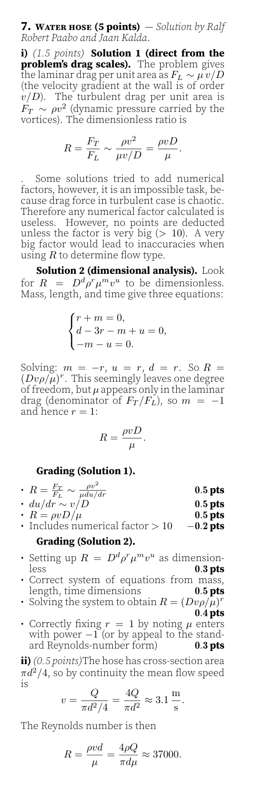
Official solution (NBPhO 2026, solutions v1.2 with grading scheme), from the official PDF; text as transcribed by olimpicos.net.
Topic: Fluid Mechanics Metodi: Dimensional Analysis, Bernoulli’s Equation, Continuity Equation Competenze: Estimation & Approximation, Mathematical Modeling Objects: Tube Fonte: Testo (PDF) — p.2 · Soluzione ufficiale (PDF)
Tubo dell’acqua (5 punti) — Ralf Robert Paabo
Un liquido di densità scorre in un tubo di diametro . A basse velocità medie il flusso è laminare (uniforme e senza vortici); la forza di attrito per unità di superficie sul liquido è dovuta all’attrito con la parete, dove (in ) è la viscosità dinamica, la velocità locale e la distanza dall’asse. Quando è abbastanza grande, il flusso diventa turbolento, pieno di vortici le cui fluttuazioni di velocità sono dell’ordine di . L’attrito è ancora dovuto all’attrito con la parete, , ma i vortici comprimono lo strato vicino alla parete (in cui la velocità passa da a zero) fino a uno spessore , tale che la forza per unità di superficie sia dell’ordine della pressione dinamica trasportata dai vortici.
i) (1,5 punti) A una data velocità domina solo uno dei due meccanismi, ma il rapporto adimensionale tra le due scale caratteristiche di attrito, , si può calcolare comunque e indica in quale regime ci si trova. Questo rapporto è il numero di Reynolds. Esprimi come prodotto di potenze di , , e .
Una pompa di potenza utile è usata per annaffiare un giardino; aspira l’acqua da una profondità direttamente in un tubo di lunghezza e diametro interno . L’acqua esce dall’estremità del tubo con portata volumetrica . La densità dell’acqua è , la viscosità e l’accelerazione di gravità .
ii) (0,5 punti) Determina il tipo di flusso nel tubo. È noto che il flusso è turbolento se e laminare altrimenti.
iii) (3 punti) Il giardiniere pulisce gli attrezzi dirigendo il getto d’acqua sulle superfici sporche. Dove il getto colpisce la superficie la pressione supera quella atmosferica; è questa sovrapressione a rimuovere lo sporco. Per pulire meglio il giardiniere monta una lancia regolata in modalità getto stretto, così che la sezione di uscita sia della sezione del tubo. Di che fattore cambia la portata volumetrica ? Di che fattore cambia la sovrapressione sulla superficie sporca? Trova entrambi con un’accuratezza dell’. Puoi usare metodi numerici.
Risposta: i) ; ii) turbolento; iii) , sovrapressione
Soluzione: La soluzione ufficiale completa (in inglese) è nella versione originale di questo quesito e nel PDF ufficiale.
Topic: Fluid Mechanics Metodi: Dimensional Analysis, Bernoulli’s Equation, Continuity Equation Competenze: Estimation & Approximation, Mathematical Modeling Objects: Tube Fonte: Testo (PDF) — p.2 · Soluzione ufficiale (PDF)
Jet sound (8 points) — Teo Kai Wen, Jaan Kalda
A fighter jet flies past a ground observer along a straight horizontal line at constant supersonic velocity, passing at closest-approach distance . The jet’s Mach number is , where is the speed of the jet and is the speed of sound. The air is at rest. The observer records the sound as a spectrogram (intensity colour-coded as a function of frequency and time; black means silence), shown below.
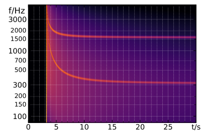
i) (2 points) Explain, qualitatively, the features seen in the spectrogram.
ii) (3 points) From the spectrogram, find the Mach number .
iii) (3 points) Find the closest-approach distance given that .
Risposta: ii) ; iii)
Soluzione:
i) (2 points) The spectrogram shows four qualitative features.
(a) Silence before . Since sound travels at a finite pace, it takes some time to hear the sound (this feature would also hold for a non-supersonic plane).
(b) Broadband spike at . An entire interval of past emissions reaches the observer simultaneously, forming a shockwave front --- the “boom” --- that registers as a short, strong pressure peak at the sensor and represents the superposition of a wide range of frequencies.
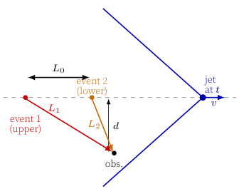
(c) Two simultaneous tones for . For each reception time (let us set ), two distinct past emission events 1 and 2 contribute. Suppose the sound from event 1, emitted at time from distance , reaches us now. Since the jet is supersonic, there is a second emission --- event 2 at a later time , distance from us, separated from event 1 by distance along the trajectory --- such that i.e., the jet’s traversal time from 1 to 2 equals the sound delay . Both arrivals are Doppler-shifted, but to different degrees: the sound coming from behind (event 1, jet far upstream and approaching the observer) is blue-shifted (upper ridge), while the sound coming from ahead (event 2, jet receding past closest approach) is red-shifted (lower ridge).
(d) Ridges decrease in time. Both ridges diverge at the boom (the broadband spike at ) and decrease monotonically afterward, tending toward finite asymptotic values as .
Grading.
-
Silence before , explained as the sound not reachin the receiver yet 0.2 pts
-
Sonic boom at , explained as the shockwave front producing a short broadband pressure peak 0.5 pts
-
Associating the changes in frequency with the Doppler effect 0.2 pts
-
Explanation of two simultaneous tones for , with two emission events reaching the observer at the same time 0.6 pts
-
Explanation of ridges diverging at the boom and tending asymptotically to finite values as 0.5 pts
ii) (3 points) As , the jet’s velocity becomes nearly aligned with the line of sight, so the radial velocity (component along the line from source to observer) approaches . The classical Doppler formula for a source moving radially at speed relative to a stationary observer is with the sign for an approaching source (, source moving toward observer) and for a receding source. Applied to the two asymptotic limits with : Combining: and , so Reading from the spectrogram: and . Therefore
Grading.
-
Recognising that the radial velocity tends to in the asymptotic limits 0.5 pts
-
Correct Doppler formula 0.5 pts
-
Asymptotic upper-ridge value 0.2 pts
-
Asymptotic lower-ridge value 0.2 pts
-
Reading and from the spectrogram (0.2p each) 0.4 pts
-
Correct symbolic form 0.8 pts
-
Numerical answer 0.4 pts
iii) (3 points) The closest-approach signal is the sound emitted when the jet’s radial velocity is zero (jet directly overhead ). At that emission, , so the received frequency equals . From part (ii)‘s asymptotic relations we have The observer hears this frequency on the lower ridge (the receding branch crosses as the jet passes overhead). Read from the spectrogram as the time when the lower ridge crosses .
Set at the moment the jet emits the sound that the observer eventually hears as the boom; call this position . Let denote the jet’s position when the observer hears the boom, and the observer. Then and the boom-tangency condition fixes (the wavefront from just grazes the observer). In particular, , identifying as the Mach angle .
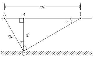
Let be the foot of perpendicular from onto trajectory , so (closest-approach distance). The right triangles and are similar (both right-angled, sharing the angle at ). From this similarity: The observer hears the boom at time and the closest-approach signal at time . The lag is Eliminating via and simplifying: Reading from the spectrogram: (boom onset) and (lower ridge crosses ), so . With :
Grading.
-
Computing with using the asymptotes from part (ii) 0.4 pts
-
Using Mach cone and the corresponding condition 0.4 pts
-
Recognising that at the point of closest approach, (no Doppler shift) 0.3 pts
-
Expressing the time between the emission (event A) and reception of the sonic boom in terms of 0.5 pts
-
Expressing the time between event A and reception of the wave emitted at B in terms of 1.0 pts
-
Reading from the spectrogram and computing 0.2 pts
-
Numerical answer if approach correct 0.2 pts
Official solution (NBPhO 2026, solutions v1.2 with grading scheme), from the official PDF; text as transcribed by olimpicos.net.
Topic: Oscillations & Waves Metodi: Wave Equation, Physical Modeling Competenze: Diagrammatic Reasoning, Experimental Data Analysis Objects: — Fonte: Testo (PDF) — p.2 · Soluzione ufficiale (PDF)
Il suono del jet (8 punti) — Teo Kai Wen, Jaan Kalda
Un caccia sorvola un osservatore a terra lungo una retta orizzontale a velocità supersonica costante, passando alla distanza minima . Il numero di Mach del jet è , dove è la velocità del jet e quella del suono. L’aria è ferma. L’osservatore registra il suono come spettrogramma (intensità codificata a colori in funzione di frequenza e tempo; il nero indica silenzio), mostrato qui sotto.
i) (2 punti) Spiega qualitativamente le caratteristiche visibili nello spettrogramma.
ii) (3 punti) Dallo spettrogramma ricava il numero di Mach .
iii) (3 punti) Trova la distanza minima sapendo che .
Risposta: ii) ; iii)
Soluzione: La soluzione ufficiale completa (in inglese) è nella versione originale di questo quesito e nel PDF ufficiale.
Topic: Oscillations & Waves Metodi: Wave Equation, Physical Modeling Competenze: Diagrammatic Reasoning, Experimental Data Analysis Objects: — Fonte: Testo (PDF) — p.2 · Soluzione ufficiale (PDF)
CO2 fire extinguisher (8 points) — Jaan Kalda
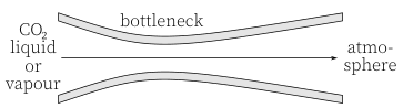
A fire extinguisher contains liquid CO in equilibrium with its saturated vapour at room temperature . Consider two scenarios: (a) the container is held upside-down so that the liquid phase flows to the nozzle; (b) it is held upright so that the saturated vapour flows to the nozzle. The nozzle has the shape of a converging—diverging channel (see figure), and the flow through it can be modelled as reversible and adiabatic. Atmospheric pressure is ; the CO triple point is at .
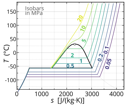
The temperature—entropy diagram of CO with isobars is provided below.
i) (1.5 points) Identify the phase or phases present and their temperature in the stream emerging from the nozzle.
ii) (3.5 points) Find the mass fraction of solid CO in the stream for both scenarios.
iii) (3 points) Now consider an arbitrary pure substance in equilibrium with its saturated vapour at temperature , and suppose that only the vapour (not the liquid) escapes through a nozzle, undergoing reversible adiabatic expansion. Under what condition on the vaporisation latent heat (per unit mass), the isobaric specific heat of the vapour , and the temperature does a fraction of the escaping vapour condense into droplets, even for a vanishingly small pressure drop? Does condensation occur for water vapour at (, )?
Risposta: ii) , ; iii) condensation iff — yes for water ()
Soluzione:
i) (1.5 points) At atmospheric pressure , which is below the triple-point pressure , no liquid CO can exist. The exit stream is therefore either pure vapour, pure solid, or a solid—vapour mixture. Pure solid is impossible: a rigid (incompressible) solid cannot expand or accelerate through a converging—diverging nozzle. So the exit is either pure vapour, or a solid—vapour mixture; in the latter case the temperature must be the sublimation temperature at 1 atm, ().
Tracing the isentrope from the initial state to bar on the — diagram (provided): for both scenarios (a) and (b), the trajectory crosses the saturation boundary into the two-phase region. Hence the stream is a solid—vapour mixture at in both cases.
Grading.
-
Recognising that liquid is impossible at , so the stream is solid, vapour, or a mixture 0.5 pts
-
Excluding pure solid (cannot adiabatically expand through nozzle) 0.2 pts
-
If solid—vapour coexistence, identifying (), within 0.3 pts
-
Tracing the isentrope on the — diagram and concluding the stream is in the two-phase region for one scenario 0.3 pts
-
Two-phase for both scenarios 0.2 pts
ii) (3.5 points) The expansion through the nozzle is reversible and adiabatic, so it is isentropic: the entropy per unit mass is conserved between the inlet and the exit. On the — diagram, the trajectory is therefore vertical (constant ) until it crosses a phase boundary or a chosen isobar.
The exit pressure is bar, well below the triple-point pressure bar. From part (i), the exit state is in the two-phase (solid+vapour) region at ().
Lever rule. In the two-phase region at fixed , , the total entropy per unit mass for a mixture with mass fraction of solid (and vapour) is where and are the entropies of pure solid and pure vapour at the boundaries of the two-phase region at bar.
Reading entropies from the — diagram. At bar (sublimation isobar at ), the boundaries are
The initial entropies for the two scenarios are read at K () on the saturation dome:
-
Scenario (a), saturated liquid at : .
-
Scenario (b), saturated vapour at : .
Mass fractions. Applying the lever rule to each:
So the liquid-fed extinguisher (a) produces a stream that is 40% dry ice (and 60% vapour) by mass, while the vapour-fed extinguisher (b) produces a stream that is only 25% dry ice. The liquid scenario yields about 1.6 times more solid CO per unit mass discharged --- which is why fire extinguishers are designed to draw liquid.
Grading.
-
Recognising that “reversible adiabatic” means isentropic (), so the end-point is found by tracing vertically downward on the — diagram 0.6 pts
-
Deriving the lever rule for mass fraction in the two-phase region: 0.7 pts
-
Reading the initial entropy from the saturated-liquid line at K (scenario a) 0.5 pts
-
Reading the initial entropy from the saturated-vapour line at (scenario b) 0.5 pts
-
Reading at the 1-bar solid boundary 0.3 pts
-
Reading at the 1-bar vapour boundary 0.3 pts
-
Computing for scenario (a) 0.3 pts
-
Computing for scenario (b) 0.3 pts
iii) (3 points) Consider an infinitesimal isentropic (reversible adiabatic) expansion of the saturated vapour from . Two trajectories meet at this point: the saturation curve , and the adiabat (constant entropy). The expansion follows the adiabat. If the adiabat falls below the saturation curve in — space (i.e., the vapour cools more slowly than the saturation temperature drops with pressure), then a finite fraction of the vapour condenses into droplets. Otherwise the expansion remains in the pure-vapour region.
Saturation slope (Clausius—Clapeyron). The saturated vapour above a liquid has number density in thermal equilibrium with the liquid. By the Boltzmann distribution, the probability of a molecule occupying the vapour state (energy per molecule above the liquid) versus the liquid state is Treating as -independent and using , the dominant temperature dependence is exponential. Per unit mass, where is the specific gas constant of the vapour. Differentiating : Equivalently,
Adiabat slope. For the ideal-gas adiabat , with and :
Condensation condition. The vapour condenses on expansion iff the adiabat cools less than the saturation curve, i.e. :
Numerical check (water at K). , :
So water vapour does condense on isentropic expansion. This is precisely why steam from a kettle appears as a visible white plume of fine droplets, rather than as invisible pure water vapour.
iv) (? points) Consider an infinitesimal isentropic (reversible adiabatic) expansion of the saturated vapour from . Two trajectories meet at this point: the saturation curve , and the adiabat (constant entropy). The expansion follows the adiabat. If the adiabat falls below the saturation curve in — space (i.e., the vapour cools more slowly than the saturation temperature drops with pressure), then a finite fraction of the vapour condenses into droplets. Otherwise the expansion remains in the pure-vapour region.
Saturation slope (Clausius—Clapeyron). The saturated vapour above a liquid has number density in thermal equilibrium with the liquid. By the Boltzmann distribution, the probability of a molecule occupying the vapour state (energy per molecule above the liquid) versus the liquid state is Treating as -independent and using , the dominant temperature dependence is exponential. Per unit mass, where is the specific gas constant of the vapour. Differentiating : Equivalently,
Adiabat slope. For the ideal-gas adiabat , with and :
Condensation condition. The vapour condenses on expansion iff the adiabat cools less than the saturation curve, i.e. :
Numerical check (water at K). , :
So water vapour does condense on isentropic expansion. This is precisely why steam from a kettle appears as a visible white plume of fine droplets, rather than as invisible pure water vapour.
Grading.
-
Setting up the comparison: condensation occurs iff the adiabat lies below the saturation curve in — space 0.5 pts
-
Deriving the saturation slope via Boltzmann: (those who know and use the Clausius—Clapeyron equation do not need to derive it) 0.6 pts
-
Obtaining the Clausius—Clapeyron form 0.6 pts
-
Adiabat slope from ideal-gas adiabatic relation 0.4 pts
-
Comparing slopes to obtain the condition 0.6 pts
-
Numerical check for water giving , hence condensation 0.3 pts
Official solution (NBPhO 2026, solutions v1.2 with grading scheme), from the official PDF; text as transcribed by olimpicos.net.
Topic: Thermodynamics Metodi: First Law of Thermodynamics, Thermodynamic Cycle Analysis Competenze: Diagrammatic Reasoning, Physical Reasoning Objects: Gas Fonte: Testo (PDF) — p.2 · Soluzione ufficiale (PDF)
Estintore a CO₂ (8 punti) — Jaan Kalda
Un estintore contiene CO liquida in equilibrio con il suo vapore saturo a temperatura ambiente . Considera due casi: (a) l’estintore è tenuto capovolto, così che verso l’ugello fluisce la fase liquida; (b) è tenuto diritto, così che verso l’ugello fluisce il vapore saturo. L’ugello ha la forma di un condotto convergente–divergente (vedi figura) e il flusso al suo interno si può modellare come reversibile e adiabatico. La pressione atmosferica è ; il punto triplo della CO è .
Qui sotto è riportato il diagramma temperatura–entropia della CO con le isobare.
i) (1,5 punti) Individua la fase o le fasi presenti nel getto che esce dall’ugello e la loro temperatura.
ii) (3,5 punti) Trova la frazione in massa di CO solida nel getto in entrambi i casi.
iii) (3 punti) Considera ora una sostanza pura qualsiasi in equilibrio con il suo vapore saturo alla temperatura , e supponi che dall’ugello esca solo il vapore (non il liquido), subendo un’espansione adiabatica reversibile. A quale condizione sul calore latente di vaporizzazione (per unità di massa), sul calore specifico a pressione costante del vapore e sulla temperatura una parte del vapore che esce condensa in goccioline, anche per una caduta di pressione piccolissima? La condensazione avviene per il vapore acqueo a (, )?
Risposta: ii) , ; iii) condensa se — sì per l’acqua ()
Soluzione: La soluzione ufficiale completa (in inglese) è nella versione originale di questo quesito e nel PDF ufficiale.
Topic: Thermodynamics Metodi: First Law of Thermodynamics, Thermodynamic Cycle Analysis Competenze: Diagrammatic Reasoning, Physical Reasoning Objects: Gas Fonte: Testo (PDF) — p.2 · Soluzione ufficiale (PDF)
Ball magnet (10 points) — Jaan Kalda
Experimental problem. Tools: ball-shaped neodymium magnet of diameter with remanence , density ; stand; permanent marker; ruler; measuring tape; flat iron disk; square wooden plate with an iron pin inserted at one side; flat wooden plate with guiding rails and non-slipping surface between them; piece of titanium of diameter and length fixed to a string. Density of titanium .
A uniformly magnetised sphere produces an external field identical to that of a point magnetic dipole with a moment , where is the sphere’s radius. Along the axis of a dipole, , where is the distance from the dipole. The dipole moment of the Earth is pointing southwards.
Warning: measure as far as possible from iron objects (table frames, chairs), which strongly perturb the geomagnetic field.
i) (2 points) Find the direction of the magnetisation of the magnet: mark on its surface a dot at the point where the straight magnetic field line exits, and a cross where it enters. Before leaving the room, give the magnet with the markings to the invigilator.
ii) (4 points) Find the magnitude of the Earth’s magnetic field at the laboratory location.
iii) (4 points) Titanium is a paramagnetic material with magnetic susceptibility . A small sample of volume in an inhomogeneous field experiences a force (‘grad’ denotes derivative in the direction of greatest change). Find for the supplied titanium wire piece.
Risposta: experimental — e.g. , (see the official solution)
Soluzione:
i) (2 points) The procedure has two stages: (1) locate the magnetic axis on the ball’s surface, and (2) determine which end is N (field exits) and which is S (field enters).
Stage 1: locate the axis. Place the ball-magnet on the flat iron disk. The magnet polarises the iron underneath, creating an attractive image-dipole. The interaction energy is minimised when the magnet’s dipole axis is perpendicular to the iron surface (so the two dipoles are aligned head-to-tail). The ball therefore rolls until its axis points straight down at the disk. With a permanent marker, mark a dot at the topmost point of the ball (where the axis exits the upper hemisphere). Then carefully invert the ball, place it on the disk again, and mark a second dot at the new topmost point. The two dots are diametrically opposite and lie on the dipole axis.
For full marking precision, the dot should be placed within 1 mm of the highest point of the ball; on a 10 mm ball this corresponds to better than angular alignment.
Stage 2: identify which dot is N. At Tallinn’s latitude, the geomagnetic field points downward into the ground (the Earth’s dipole moment points southwards as stated, so its field lines re-enter the ground in the northern hemisphere). A free magnet self-orients with . Place the ball on the flat wooden plate (well away from iron objects). The geomagnetic torque rotates the ball until its dipole moment aligns with --- pointing downward, predominantly. The ball does not roll away: itself holds the ball in the aligned orientation, since once the torque vanishes.
The N pole (where exits, head of ) is then on the bottom of the ball, and the S pole on top. Re-mark the upward-pointing dot with a cross (): this is the S pole where enters. Leave the downward-pointing dot as a dot: this is the N pole where exits.
Grading.
Method:
-
Realising that the magnet rolls so its axis is perpendicular to the iron disk 0.5 pts
-
Recognising that the geomagnetic field at Tallinn points downward into the ground 0.5 pts
-
Realising that the free magnet self-orients with , hence N points downward 0.5 pts
Experiment:
-
Procedure to mark both poles (dot on top, invert, dot on top again, giving two diametrically opposite axis-points) 0.2 pts
-
Both dots placed within 1 mm of the true axis-exit points 0.1 pts
-
Correctly marking the upward-pointing dot as a cross (S, field enters) and leaving the downward dot (N, field exits) 0.2 pts
ii) (4 points) Idea. Place the ball-magnet between the rails on the wooden plate. As the plate is tilted, gravity tries to roll the ball downhill (rotating away from ), while exerts a restoring magnetic torque trying to keep aligned. At a critical tilt , gravity overcomes the maximum magnetic restoring torque, and the ball begins to roll. Measuring gives .
Setup. The cross on the ball is slightly displaced from the exact top because is tilted from vertical (dip angle in Tallinn, so the horizontal component of is non-zero and points magnetic-north). Orient the plate so that the cross’s small horizontal offset from the topmost point lies parallel to the rails. Equivalently, the rails should run along the magnetic meridian, with the ball’s dipole axis lying in the vertical plane containing and the rolling direction.
Procedure.
-
Place the plate horizontally and let the ball settle: it self-orients with , with the cross slightly offset toward magnetic-south of the topmost point.
-
Re-orient the plate (in the horizontal plane) so the cross’s offset is parallel to the rails (cross equidistant from both rails).
-
Slowly tilt one end of the plate upward. Measure the elevation of the higher end above the lower end with the ruler; for a plate of length , the tilt angle satisfies .
-
Continue tilting smoothly and slowly until the ball just begins to roll down. Record at that instant.
-
Lower the plate, slightly displace the ball to reset, allow re-orientation, repeat. Average over many trials --- readings fluctuate due to small variations in initial alignment, friction at the rails, and the smoothness of tilting.
Force/torque balance. Just before rolling, the ball is in static equilibrium between gravity and the magnetic restoring torque. The gravitational torque about the ball’s center (acting through the rail contact at distance ) is , where is the ball radius. The maximum magnetic restoring torque (when ) is . Critical condition:
The magnet’s dipole moment is , with mass . So
Measurements. A representative set of trials with rail length :
| trial | 1 | 2 | 3 | 4 | 5 | 6 | 7 | 8 | 9 | 10 | avg |
|---|---|---|---|---|---|---|---|---|---|---|---|
| (mm) | 24 | 26 | 25 | 27 | 23 | 25 | 26 | 24 | 25 | 25 | 25.0 |
The standard deviation of the readings is , giving a standard error on the mean of , or about 1.5% of the average.
With :
Combined uncertainty (statistical from plus systematic from and at the few-percent level): , in good agreement with the known geomagnetic field at Tallinn’s latitude (50 T).
Grading.
-
Recognising that gravity drives rolling and magnetic torque resists it 0.2 pts
-
Gravity torque on ball: (force times lever arm to contact line) 0.2 pts
-
Maximum magnetic torque (when ) 0.3 pts
-
Procedure: tilt the plate and record the critical angle when the ball begins to roll 0.4 pts
-
Realising that the rails should be aligned with the cross’s horizontal offset (i.e., parallel to the magnetic meridian) 0.4 pts
-
Critical-condition formula 0.5 pts
-
Solving for 0.3 pts
-
Computing from the given and ball geometry 0.4 pts
-
Documented measurements (multiple trials, table or list of readings) with averaging and uncertainties 0.8 pts
-
Plausible numerical answer for in the range to 0.5 pts
iii) (4 points) Setup. The titanium piece hangs as a pendulum from a string of length attached to the stand. Bring the ball-magnet close to the Ti so that one of its poles touches the Ti’s surface. The paramagnetic Ti is attracted toward the magnet. Slowly and smoothly pull the magnet-and-Ti combination horizontally; the pendulum tilts. At a critical horizontal displacement , the magnetic attraction can no longer balance the gravitational restoring force, and the Ti detaches from the magnet and swings back. Measuring gives .
Practical execution.
-
Keep the magnet stuck to the iron pin in the wooden plate as a holder, so it always points one pole forward (rather than rotating in the hand).
-
Ensure the magnet’s pole touches the Ti at all times and at the same point (the magnet’s tip, on the dipole axis); a slight shift up or down reduces the magnetic force.
-
Pull very slowly so the system is quasi-static (no inertial effects, ).
-
Repeat many times. Take the maximum observed as the result; smaller readings reflect imperfect execution (acceleration, off-axis contact, etc.).
A typical observed range: to .
Physics. The ball-magnet has dipole moment . On its dipole axis, at distance from the centre,
At the moment of contact with the Ti, the smallest distance from the magnet’s center to the Ti’s center is .
The force on the paramagnetic Ti, using the formula given in the problem with and :
Force balance at detachment. Just before the Ti detaches, the pendulum’s tilt angle satisfies , and the horizontal restoring force is . Setting this equal to the maximum magnetic force (at ):
Using to cancel :
Numerical evaluation. Take pendulum length (estimated from the stand) and (representative maximum from many trials). Then , . With :
This is consistent with the literature value for pure titanium (), within the precision afforded by the experimental uncertainties.
Grading.
-
Setup: pendulum + magnet, identification of detachment as the limit condition 0.3 pts
-
Practical execution detail: keep magnet on iron pin to maintain orientation 0.2 pts
-
Practical execution detail: ensure pole touches Ti at the same axial point 0.2 pts
-
Practical execution detail: pull slowly (quasi-static, ) 0.2 pts
-
Performing measurements (either stated explicitly that the reported value is the maximum of trials, or measurements documented in a table/list) 0.4 pts
-
Taking the maximum (not average) of the measurements as the reported 0.4 pts
-
Combining the given dipole-field and paramagnetic-force formulas into 0.3 pts
-
Identifying as magnet radius + Ti half-thickness (accounting for the wire’s radius) 0.4 pts
-
Force balance (or equivalently if the magnet is pulled perpendicular to the thread rather than strictly horizontally; the two forms differ by 3% at the critical angle, smaller than experimental scatter; both can be approximated as ) 0.5 pts
-
Solving this equation for 0.3 pts
-
Documenting the observed maximum . Full credit for ; reduce by 0.1 pts per half a degree outside this range, down to a minimum of 0 0.3 pts
-
Numerical answer for . Full credit for ; reduce by 0.1 pts for each outside this range, down to a minimum of 0 0.5 pts
Grading note (default credit for execution details): if the three execution details (iron-pin holder, axial pole contact, slow quasi-static pulling) are not stated explicitly but the reported maximum horizontal displacement is at least , award 50% of each item’s points (0.1 pts each, keep one decimal). The reasoning: a result in this range can only be obtained if execution was acceptable, even if the student didn’t articulate why.
Official solution (NBPhO 2026, solutions v1.2 with grading scheme), from the official PDF; text as transcribed by olimpicos.net.
Topic: Magnetism Metodi: Experimental Data Analysis, Torque & Angular Momentum Analysis Competenze: Measurement & Instrumentation, Experimental Data Analysis Objects: Magnet, Magnetic Dipole Fonte: Testo (PDF) — p.2 · Soluzione ufficiale (PDF)
Magnete sferico (10 punti) — Jaan Kalda
Problema sperimentale. Materiale: magnete sferico al neodimio di diametro con magnetizzazione residua e densità ; supporto; pennarello indelebile; righello; metro a nastro; disco di ferro piatto; tavoletta quadrata di legno con un perno di ferro inserito su un lato; tavoletta piana di legno con guide e superficie antiscivolo tra di esse; pezzetto di titanio di diametro e lunghezza fissato a un filo. Densità del titanio .
Una sfera magnetizzata uniformemente produce all’esterno lo stesso campo di un dipolo magnetico puntiforme di momento , dove è il raggio della sfera. Lungo l’asse di un dipolo , dove è la distanza dal dipolo. Il momento di dipolo della Terra è diretto verso sud.
Attenzione: misura il più lontano possibile da oggetti di ferro (telai dei tavoli, sedie), che perturbano fortemente il campo geomagnetico.
i) (2 punti) Trova la direzione della magnetizzazione del magnete: segna sulla sua superficie un punto dove esce la linea di campo rettilinea e una croce dove entra. Prima di lasciare l’aula consegna il magnete con i segni al sorvegliante.
ii) (4 punti) Trova il modulo del campo magnetico terrestre nel luogo del laboratorio.
iii) (4 punti) Il titanio è un materiale paramagnetico con suscettività magnetica . Un piccolo campione di volume in un campo non uniforme subisce una forza (“grad” indica la derivata nella direzione di massima variazione). Trova per il pezzetto di filo di titanio fornito.
Risposta: sperimentale — ad es. , (vedi la soluzione ufficiale)
Soluzione: La soluzione ufficiale completa (in inglese) è nella versione originale di questo quesito e nel PDF ufficiale.
Topic: Magnetism Metodi: Experimental Data Analysis, Torque & Angular Momentum Analysis Competenze: Measurement & Instrumentation, Experimental Data Analysis Objects: Magnet, Magnetic Dipole Fonte: Testo (PDF) — p.2 · Soluzione ufficiale (PDF)
Final results from the official NBPhO 2026 solutions (v1.2).
| Problem | Title | Risposta |
|---|---|---|
| 1 | Moving lens (6 points) — Eppu Leinonen | geometric construction — see the official solution |
| 2 | Lissajous bridge (6 points) — Jaan Kalda | |
| 3 | Kirill on a swing (8 points) — Kaarel Hänni | iii) stand-ups () |
| 4 | Rod and bead (8 points) — Eero Ristolainen, Jaan Kalda | ii) ; iii) , ; iv) , , |
| 5 | Saturation pressure of water (8 points) — Eero Uustalu | experimental — e.g. at (see the official solution) |
| 6 | Pull-up bar rope (5 points) — Jaan Kalda | i) ; ii) ; iii) |
| 7 | Water hose (5 points) — Ralf Robert Paabo | i) ; ii) turbulent; iii) , excess pressure |
| 8 | Jet sound (8 points) — Teo Kai Wen, Jaan Kalda | ii) ; iii) |
| 9 | CO2 fire extinguisher (8 points) — Jaan Kalda | ii) , ; iii) condensation iff — yes for water () |
| 10 | Ball magnet (10 points) — Jaan Kalda | experimental — e.g. , (see the official solution) |
Fonte: Testo e soluzioni (PDF)
Risultati finali dalle soluzioni ufficiali NBPhO 2026 (v1.2).
| Problema | Titolo | Risposta |
|---|---|---|
| 1 | Lente in movimento (6 punti) — Eppu Leinonen | costruzione geometrica — vedi la soluzione ufficiale |
| 2 | Ponte di Lissajous (6 punti) — Jaan Kalda | |
| 3 | Kirill sull’altalena (8 punti) — Kaarel Hänni | iii) volte () |
| 4 | Asta e perlina (8 punti) — Eero Ristolainen, Jaan Kalda | ii) ; iii) , ; iv) , , |
| 5 | Tensione di vapore saturo dell’acqua (8 punti) — Eero Uustalu | sperimentale — ad es. a (vedi la soluzione ufficiale) |
| 6 | La fune sulla sbarra (5 punti) — Jaan Kalda | i) ; ii) ; iii) |
| 7 | Tubo dell’acqua (5 punti) — Ralf Robert Paabo | i) ; ii) turbolento; iii) , sovrapressione |
| 8 | Il suono del jet (8 punti) — Teo Kai Wen, Jaan Kalda | ii) ; iii) |
| 9 | Estintore a CO₂ (8 punti) — Jaan Kalda | ii) , ; iii) condensa se — sì per l’acqua () |
| 10 | Magnete sferico (10 punti) — Jaan Kalda | sperimentale — ad es. , (vedi la soluzione ufficiale) |
Fonte: Testo e soluzioni (PDF)