OPhO 2024 — Invitational Experimental

2024 OPhO Experimental Exam: Ising Model of Ferromagnetism (August 30 – September 1)

Introduction

Paramagnetic materials have atoms with permanent magnetic dipoles, but point in random directions unless aligned by an external magnetic field. On the other hand, magnetic dipoles in ferromagnetic materials align with neighboring dipoles and can have a significant magnetization even without an external field.

Iron is one common example of a material that is ferromagnetic at room temperature. Other materials undergo a phase transition, where they are paramagnetic at higher temperatures, but become ferromagnetic below a certain temperature (the Curie temperature, $T_{c}$ ).

In this experiment, we will use the Ising Model and a Monte Carlo simulation to compute and examine the properties of this phase transition.

The Ising Model is a simple approximation for ferromagnetism. We take a 2D lattice of atoms and assume that each dipole points either up ( $s_{i} = 1$ ) or down ( $s_{i} = - 1$ ) along the same axis. Then we run the Monte Carlo simulation, which uses the following algorithm:

Start with a 2D grid of size $L \times L$ , where each site represents a spin that can be either $+ 1$ or $- 1$ . The initial configuration is randomly assigned.
Energy Calculation: For each spin at position $(i, j)$ , calculate the change in energy ( $Δ E$ ) if the spin is flipped. This is done by considering the interaction of the spin with its nearest neighbors. The energy change $Δ E$ (in the absence of an external field) is given by:

$Δ E = 2 J \times spin \times (\sum_{neighbors} spin)$

where $J$ is the interaction strength.

For each Monte Carlo step:
- Randomly select a spin in the grid.
- Calculate the energy change $Δ E$ if this spin were to be flipped.
- If $Δ E < 0$ , flip the spin.
- If $Δ E \geq 0$ , flip the spin with probability $e^{- Δ E / k_{B} T}$ , where $T$ is the temperature and $k_{B}$ is the Boltzmann constant.
Repeat the spin-flipping process for a set number of steps, allowing the system to reach equilibrium.
The final configuration of the grid after the simulation, representing the state of the system at temperature $T$ .

Accessing the Program

To access the Python notebook, follow this link and make a copy to your own Google Drive. You will be able to perform all the code online without needing to download anything.

Overview of Code

There are three cells to run experiments:

Varying the temperature via T_list which contains all of the simulated temperatures.
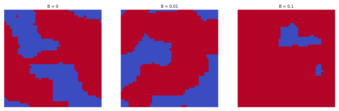
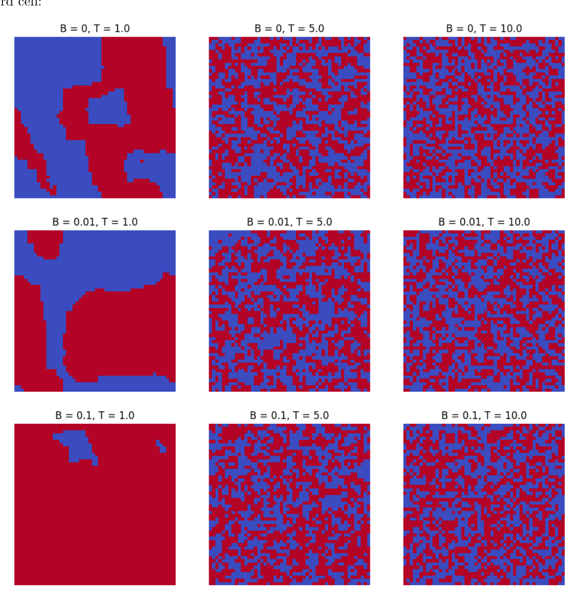
Varying the external magnetic field via B_list which contains all of the simulated external fields.
Varying both.

Instructions for Using the Simulation

The simulation uses a 50x50 grid to represent the 2D lattice of atoms. This grid is periodic, meaning that it wraps around at the edges, allowing for continuous boundary conditions.
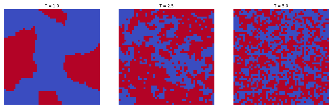
You can simulate the system at different temperatures by adjusting the T_list or B_list variable (based on desired experiment) in the code. The default temperatures provided are 1.0, 2.5, and 5.0.
The number of Monte Carlo steps can be modified by changing the n_steps variable. The default is set to 100,000 steps, but you may increase or decrease this based on your needs.
The interaction strength ( $J$ ) and Boltzmann constant ( $k_{B}$ ) are set to 1.0 by default. It is recommended not to change these values as they are critical to maintaining the accuracy of the model.
Once you’ve adjusted the parameters, run the cells in the notebook to simulate the Ising Model at the chosen temperatures. The results will be visualized, showing the spin configuration of the grid for each temperature.

Below is an image of what the initial simulation should look like for the first cell:

For the second cell:

For the third cell:

Phase Transition

For the following questions, include the figure with uncertainty if applicable, your reasoning, and any graphs if used.

a) Find the value of $T_{c}$ and explain what criteria you used.

b) Keeping the external magnetic field constant, plot the energy $E$ of the system as a function of temperature.

c) Plot the heat capacity $C$ of the system as a function of temperature. What are its maximum and minimum values?

A phase transition is first order in temperature if the energy is discontinuous, second order if the energy is continuous but its first derivative is discontinuous, etc. What is the order of the phase transition here?

Consider the net magnetization $M = μ \sum_{i = 1}^{N} s_{i}$ of the system.

d) At temperatures slightly below $T_{c}$ , $M$ can be approximated as $M = α ∣ T_{c} - T ∣^{β}$ . Find values for $α$ and $β$ .

e) Set $T = T_{c}$ . Plot how the net magnetization reacts as $B$ is varied. Qualitatively, what do you observe? What happens if $T < T_{c}$ ?

Fonte: Testo (PDF) — p.1

Topic: Thermodynamics, Magnetism Metodi: Statistical Averaging, Experimental Data Analysis, Differential Equations Competenze: Experimental Data Analysis, Mathematical Modeling Objects: Magnetic Dipole

Esame sperimentale di OPhO: Modello di ising del ferromagnetismo (MSK1/) (2024 OPhO Exam: Ising Model of Ferromagnetism)

Introduzione

I materiali paramagnetistici hanno atomi con dipoli magnetici permanenti, ma puntano in direzioni casuali a meno che non siano allineati da un campo magnetico esterno. D’altra parte, i dipoli magnetici nei materiali ferromagnetici si allineano con i dipoli vicini e possono avere una significativa magnetizzazione anche senza un campo esterno.

Il ferro è un esempio comune di materiale ferromagnetico a temperatura ambiente. Altri materiali subiscono una transizione di fase, in cui sono paramagneticamente ad alte temperature, ma diventano ferromagneticamente al di sotto di una certa temperatura (temperatura di Curie, $T_{c}$ ).

In questo esperimento, useremo il modello Ising e una simulazione di Monte Carlo per calcolare e esaminare le proprietà di questa transizione di fase.

Il modello di Ising è un’approssimazione semplice per il ferromagnetismo. Prendiamo una rete 2D di atomi e supponiamo che ogni dipolo punta su ( $s_{i} = 1$ ) o giù ( $s_{i} = - 1$ ) lungo lo stesso asse. Quindi eseguiamo la simulazione di Monte Carlo, che utilizza il seguente algoritmo:

Inizia con una griglia 2D di dimensioni $L \times L$ , dove ogni sito rappresenta uno spin che può essere $+ 1$ o $- 1$ . La configurazione iniziale è assegnata a caso.
**Calcolo dell’energia: ** Per ogni rotazione in posizione $(i, j)$ , calcolare il cambiamento di energia ( $Δ E$ ) se la rotazione è ribaltata. Questo viene fatto considerando l’interazione del spin con i suoi vicini più vicini. Il cambiamento di energia $Δ E$ (in assenza di un campo esterno) è dato da:

$Δ E = 2 J \times spin \times (\sum_{neighbors} spin)$

dove $J$ è la forza di interazione.

Per ogni passo di Monte Carlo:

Selezionate un giro in griglia.
Calcolare il cambiamento di energia $Δ E$ se si inversa questo giro.
Se $Δ E < 0$ , inversa la rotazione.
Se $Δ E \geq 0$ , inversione della rotazione con probabilità $e^{- Δ E / k_{B} T}$ , dove $T$ è la temperatura e $k_{B}$ è la costante di Boltzmann.

Ripetere il processo di spinning-flipping per un determinato numero di passaggi, consentendo al sistema di raggiungere l’equilibrio.
La configurazione finale della griglia dopo la simulazione, che rappresenta lo stato del sistema a temperatura $T$ .

Accedere al programma

Per accedere al notebook Python, segui questo link e fai una copia sul tuo Google Drive. Potrai eseguire tutto il codice online senza dover scaricare nulla.

Overview del codice

Ci sono tre cellule per eseguire esperimenti:

Variazione della temperatura via T_list che contiene tutte le temperature simulate.
Variazione del campo magnetico esterno tramite B_list che contiene tutti i campi esterni simulati.
- Variazione delle due.

Instruzioni per l’uso della simulazione

La simulazione utilizza una griglia 50x50 per rappresentare la rete 2D di atomi. Questa griglia è periodica, il che significa che si avvolge ai bordi, consentendo condizioni di confine continue.
Si può simulare il sistema a diverse temperature regolaendo la variabile T_list o B_list (in base all’esperimento desiderato) nel codice. Le temperature predefinite fornite sono 1.0, 2.5 e 5.0.
Il numero di passi di Monte Carlo può essere modificato modificando la variabile n_steps. La definizione predefinita è di 100.000 passi, ma puoi aumentare o diminuire in base alle tue esigenze.
La forza di interazione ( $J$ ) e la costante di Boltzmann ( $k_{B}$ ) sono impostate a 1,0 per impostazione predefinita. Si raccomanda di non modificare questi valori in quanto sono fondamentali per mantenere l’accuratezza del modello.
Una volta che hai regolato i parametri, eseguire le celle nel notebook per simulare il modello di Ising alle temperature scelte. I risultati saranno visualizzati, mostrando la configurazione di spin della griglia per ogni temperatura.

Di seguito è riportata un’immagine di come dovrebbe essere la simulazione iniziale per la prima cella:

Per la seconda cella:

Per la terza cella:

Transizione di fase

Per le seguenti domande, inserisci la cifra con incertezza se del caso, il tuo ragionamento e eventuali grafici se del caso.

**a) ** Trova il valore di $T_{c}$ e spiega quali criteri hai utilizzato.

**b) ** Tenendo costante il campo magnetico esterno, tracciare l’energia $E$ del sistema in funzione della temperatura.

**c) ** Indicare la capacità termico $C$ del sistema in funzione della temperatura. Quali sono i valori massimi e minimi?

Una transizione di fase è di primo ordine di temperatura se l’energia è discontinuo, di secondo ordine se l’energia è continua ma la sua prima derivata è discontinuo, ecc. Qual è l’ordine della transizione di fase qui?

Considerate la magnetizzazione netta $M = μ \sum_{i = 1}^{N} s_{i}$ del sistema.

**d) ** A temperature leggermente inferiori a $T_{c}$ , $M$ può essere approssimato a $M = α ∣ T_{c} - T ∣^{β}$ . Trova i valori per $α$ e $β$ .

**e) ** Set $T = T_{c}$ . Tracciare come la magnetizzazione netta reagisce come $B$ è variabile. Qualitativamente, cosa osservate? Che cosa succede se $T < T_{c}$ ?