PLANCKS 2014 — Utrecht

Graphene — Carlo Beenakker, Leiden University

Graphene is a mono-atomic layer of carbon atoms, arranged in a honeycomb lattice. Conduction electrons move in the $(x,y)$-plane of the layer, with velocity $v=10^{6}m/s$ that is independent of their energy $E$.

[1] 2 points Explain why the conduction electrons in graphene are called “massless particles”.

Because the honeycomb lattice has two atoms in the unit cell, the wave function of the conduction electrons has two components ${\Psi }_1(x,y)$ and ${\Psi }_2(x,y)$. The two components satisfy a pair of coupled quantum mechanical wave equations,

$$\{\begin{array}{l}U(x,y){\Psi }_1(x,y)+(v{p}_x-iv{p}_y){\Psi }_2(x,y)=E{\Psi }_1(x,y),\\ U(x,y){\Psi }_2(x,y)+(v{p}_x+iv{p}_y){\Psi }_1(x,y)=E{\Psi }_2(x,y).\end{array}$$

The electrical potential energy is indicated by $U(x,y)$ and $p_x=-i\hslash \partial /\partial x$, $p_y=-i\hslash \partial /\partial y$ are the two components of the momentum operator. For a uniform potential $U(x,y)\equiv U_0$ the solutions are proportional to the plane wave $\exp (i{k}_{x}x+i{k}_{y}y)$.

[2] 4 points Derive, for this case of uniform potential $U_0$, the relation between the energy $E$ and the wave vector components $k_x,k_y$. Make a plot of $E$ as a function of $k\equiv \sqrt{k_x^2+k_y^2}$. The singularity at $k=0$ is called “conical point” or “Dirac point”, and is a unique feature of graphene.

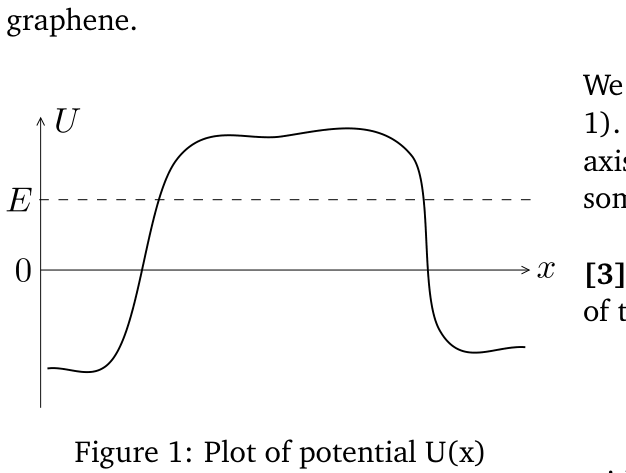Figure 1: Plot of potential $U(x)$.

We introduce a potential barrier $U(x)$ (see Figure 1). An electron moves at energy $E$ along the $x$-axis towards the barrier and is reflected by it with some probability $R$.

[3] 4 points Verify this ($y$-independent) solution of the wave equation:

$$\{\begin{array}{l}{\Psi }_1(x)=C\exp \left(\frac{i}{v\hslash }{\int }_0^x[E-U(x^{\prime })]d{x}^{\prime }\right)\\ {\Psi }_2(x)=s{\Psi }_1(x)\end{array}$$

with $C$ an arbitrary constant and $s$ equal to $+1$ or $-1$.

[4] 3 points Show that the reflection probability $R=0$ at any energy no matter how high the potential barrier. This surprising result is known as the Klein paradox.

Fonte: Testo (PDF) — p.6 Topic: Modern-Quantum Physics, Electromagnetism Metodi: Differential Equations, de Broglie Relation, Symmetry Argument Competenze: Mathematical Modeling, Physical Reasoning Objects: Electron

Grafene — Carlo Beenakker, Leiden University

Il grafene è uno strato monoatomico di atomi di carbonio, disposti in un reticolo a nido d’ape. Gli elettroni di conduzione si muovono nel piano $(x,y)$ dello strato, con velocità $v=10^{6}m/s$ indipendente dalla loro energia $E$.

[1] 2 punti Spiega perché gli elettroni di conduzione nel grafene sono chiamati “particelle prive di massa”.

Poiché il reticolo a nido d’ape ha due atomi nella cella unitaria, la funzione d’onda degli elettroni di conduzione ha due componenti ${\Psi }_1(x,y)$ e ${\Psi }_2(x,y)$. Le due componenti soddisfano una coppia di equazioni d’onda quantomeccaniche accoppiate,

$$\{\begin{array}{l}U(x,y){\Psi }_1(x,y)+(v{p}_x-iv{p}_y){\Psi }_2(x,y)=E{\Psi }_1(x,y),\\ U(x,y){\Psi }_2(x,y)+(v{p}_x+iv{p}_y){\Psi }_1(x,y)=E{\Psi }_2(x,y).\end{array}$$

L’energia potenziale elettrica è indicata con $U(x,y)$ e $p_x=-i\hslash \partial /\partial x$, $p_y=-i\hslash \partial /\partial y$ sono le due componenti dell’operatore quantità di moto. Per un potenziale uniforme $U(x,y)\equiv U_0$ le soluzioni sono proporzionali all’onda piana $\exp (i{k}_{x}x+i{k}_{y}y)$.

[2] 4 punti Ricava, per questo caso di potenziale uniforme $U_0$, la relazione tra l’energia $E$ e le componenti del vettore d’onda $k_x,k_y$. Traccia un grafico di $E$ in funzione di $k\equiv \sqrt{k_x^2+k_y^2}$. La singolarità in $k=0$ è chiamata “punto conico” o “punto di Dirac”, ed è una caratteristica peculiare del grafene.

Figure 1: Plot of potential $U(x)$.

Introduciamo una barriera di potenziale $U(x)$ (vedi Figura 1). Un elettrone si muove con energia $E$ lungo l’asse $x$ verso la barriera e viene da essa riflesso con una certa probabilità $R$.

[3] 4 punti Verifica questa soluzione (indipendente da $y$) dell’equazione d’onda:

$$\{\begin{array}{l}{\Psi }_1(x)=C\exp \left(\frac{i}{v\hslash }{\int }_0^x[E-U(x^{\prime })]d{x}^{\prime }\right)\\ {\Psi }_2(x)=s{\Psi }_1(x)\end{array}$$

con $C$ una costante arbitraria e $s$ uguale a $+1$ o $-1$.

[4] 3 punti Mostra che la probabilità di riflessione $R=0$ a qualsiasi energia, per quanto alta sia la barriera di potenziale. Questo risultato sorprendente è noto come paradosso di Klein.

Fonte: Testo (PDF) — p.6 Topic: Modern-Quantum Physics, Electromagnetism Metodi: Differential Equations, de Broglie Relation, Symmetry Argument Competenze: Mathematical Modeling, Physical Reasoning Objects: Electron

Newton’s Cradle — Jan van Ruitenbeek, Leiden University

Figure 2: Newton’s Cradle.

Newton’s cradle is a well-known gadget and physics demonstration. It is usually described as demonstrating the laws of conservation of energy and conservation of momentum. For simplicity we take the motion to be one-dimensional and the collisions to be elastic.

[1] 5 points We launch a single ball onto the other balls that are at rest, and consider the situation just after the collision. For any number $N$ of balls (including the launched ball) in the cradle how many solutions do the laws of conservation of energy and momentum permit? For $N=2$ and $N=3$ describe the set of allowed solutions in $N$-dimensional velocity space.

[2] 5 points When we perform the experiment for $N=3$ we find that only one solution is realised. Which solution is this, and explain why.

Fonte: Testo (PDF) — p.7 Topic: Conservation of Momentum, Conservation of Energy Metodi: Conservation of Momentum, Conservation of Energy, Conservation Laws Competenze: Physical Reasoning, Mathematical Modeling Objects: Ball

Cradle di Newton Jan van Ruitenbeek, Università di Leiden

Figura 2: Culla di Newton.

La culla di Newton è un’apparecchiatura ben nota e una dimostrazione di fisica. Di solito viene descritto come dimostrando le leggi della conservazione dell’energia e della conservazione dell’impulso. Per semplicità, il movimento è unidimensional e le collisioni elastic.

** [1] ** *5 punti * Lanciamo una sola palla sulle altre palle che sono in riposo, e consideriamo la situazione subito dopo la collisione. For any number $N$ of balls (including the launched ball) in the cradle how many solutions do the laws of conservation of energy and momentum permit? Per $N=2$ e $N=3$ descrivere l’insieme delle soluzioni consentite nello spazio di velocità dimensionale $N$.

[2] 5 punti Quando eseguiamo l’esperimento per $N=3$ troviamo che si ottiene solo una soluzione. Qual è la soluzione e spiegate il perché.

Fonte: Testo (PDF) — p.7 Topic: Conservation of Momentum, Conservation of Energy Metodi: Conservation of Momentum, Conservation of Energy, Conservation Laws Competenze: Physical Reasoning, Mathematical Modeling Objects: Ball

2DEG at the AlGaAs-GaAs interface — Ingmar Swart, Utrecht University

A 2-dimensional electron gas (2DEG) can exist at the interface between semiconductors. One example where this naturally occurs is at the AlGaAs-GaAs interface. Due to the bending of the energy bands, the potential energy landscape has the shape as shown by the dashed line in Figure 3. To first order, the area where the 2DEG forms, can be approximated by a triangular shaped potential well: $V(x<0)=\infty$ and $V(x>0)=Fx$, where $F$ is a proportionality constant which has dimensions of force. It will be of the order of $10\frac{\mathrm{meV}}{\mathrm{nm}}$, or $1\mathrm{pN}$. In this case, the problem can be solved analytically.

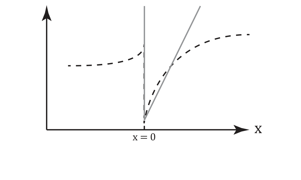Figure 3: Schematic illustration of the potential energy landscape of a AlGaAs-GaAs interface (black dashed line). The area where the 2DEG is formed can be approximated by a triangular barrier (gray solid line).

For the wavefunction, use the ansatz where $k$ is the wave vector.

$$\{\begin{array}{ll}{\psi }_k(x)=x{e}^{-kx/2}& \text{For }x\ge 0\\ {\psi }_k(x)=0& \text{For }x<0\end{array}$$

[1] 10 points Show that the expectation value of the ground state energy using this ansatz is given by:

$$E_g=2.48{\left(\frac{{\hslash }^2}{2m^{\ast }}\right)}^{1/3}{F}^{2/3}$$

with $m^{\ast }$ the effective mass. You may find the following integral helpful.

$${\int }_0^{\infty }{x}^n{e}^{kx}dx=(-1{)}^n\frac{d^n}{d{k}^n}{\int }_0^{\infty }{e}^{-kx}dx=\frac{n!}{k^{n+1}}$$

Fonte: Testo (PDF) — p.8 Topic: Modern-Quantum Physics, Mathematics Metodi: Calculus-Integration, Energy Conservation Method, Dimensional Analysis Competenze: Mathematical Modeling, Physical Reasoning Objects: Electron

2DEG all’interfaccia AlGaAs-GaAs — Ingmar Swart, Utrecht University

Un gas di elettroni bidimensionale (2DEG) può esistere all’interfaccia tra semiconduttori. Un esempio in cui ciò avviene naturalmente è l’interfaccia AlGaAs-GaAs. A causa della curvatura delle bande energetiche, il profilo di energia potenziale ha la forma mostrata dalla linea tratteggiata nella Figura 3. In prima approssimazione, la regione in cui si forma il 2DEG può essere approssimata da una buca di potenziale a forma triangolare: $V(x<0)=\infty$ e $V(x>0)=Fx$, dove $F$ è una costante di proporzionalità che ha le dimensioni di una forza. Essa sarà dell’ordine di $10\frac{\mathrm{meV}}{\mathrm{nm}}$, ovvero $1\mathrm{pN}$. In questo caso, il problema può essere risolto analiticamente.

Figure 3: Schematic illustration of the potential energy landscape of a AlGaAs-GaAs interface (black dashed line). The area where the 2DEG is formed can be approximated by a triangular barrier (gray solid line).

Per la funzione d’onda, usa l’ansatz seguente, in cui $k$ è il vettore d’onda.

$$\{\begin{array}{ll}{\psi }_k(x)=x{e}^{-kx/2}& \text{For }x\ge 0\\ {\psi }_k(x)=0& \text{For }x<0\end{array}$$

[1] 10 punti Mostra che il valore di aspettazione dell’energia dello stato fondamentale ottenuto con questo ansatz è dato da:

$$E_g=2.48{\left(\frac{{\hslash }^2}{2m^{\ast }}\right)}^{1/3}{F}^{2/3}$$

con $m^{\ast }$ la massa efficace. Il seguente integrale potrebbe esserti utile.

$${\int }_0^{\infty }{x}^n{e}^{kx}dx=(-1{)}^n\frac{d^n}{d{k}^n}{\int }_0^{\infty }{e}^{-kx}dx=\frac{n!}{k^{n+1}}$$

Fonte: Testo (PDF) — p.8 Topic: Modern-Quantum Physics, Mathematics Metodi: Calculus-Integration, Energy Conservation Method, Dimensional Analysis Competenze: Mathematical Modeling, Physical Reasoning Objects: Electron

Exercises on Particle Physics — André Mischke, Utrecht University

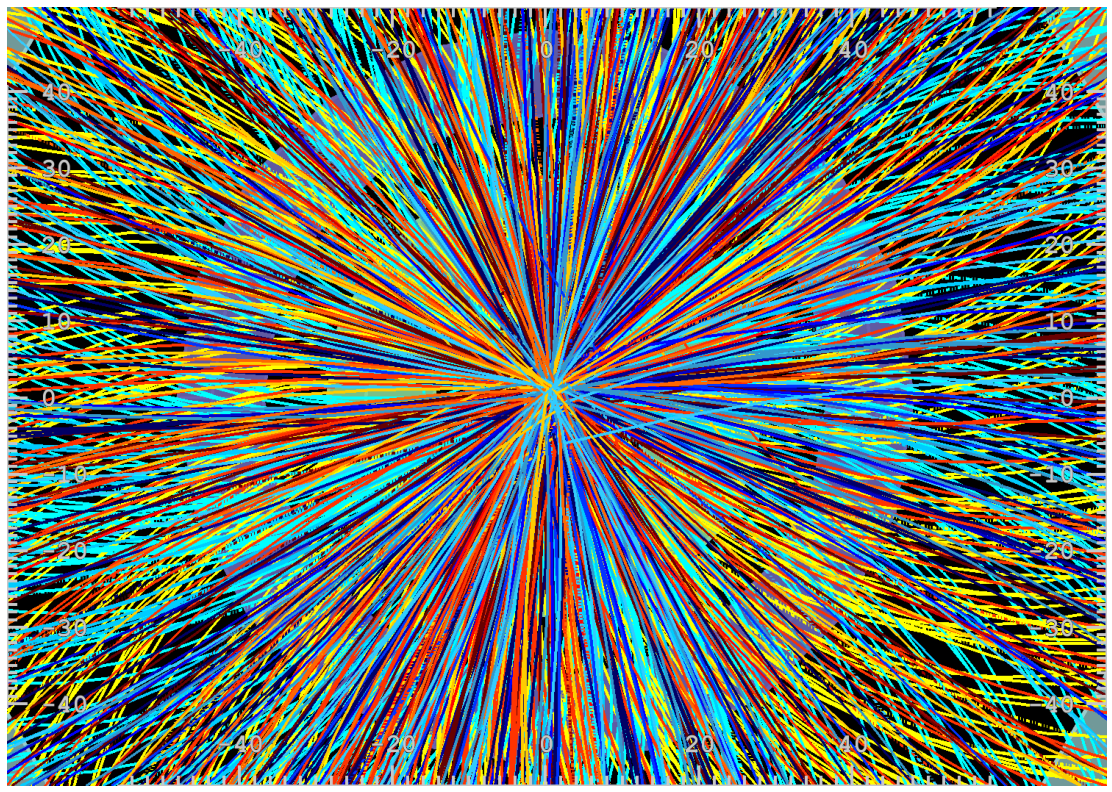Figure 4: Tracks of particles from a collision of lead atomic nuclei, reconstructed by the ALICE experiment at the CERN Large Hadron Collider.

Charged particles in magnetic fields

[1] 2 points A proton beam with a kinetic energy of $200\mathrm{GeV}$ passes through a $2\mathrm{m}$ long dipole magnet with a field strength of $2\mathrm{T}$. Calculate the deflection angle $\Theta$ of the beam using the relation $2\sin \frac{\Theta }{2}=L/R$ and the momentum $p=0.3\cdot qBR$, where $L$ is the length, $R$ the radius, $q$ the charge, and $B$ the magnetic field. The mass of the proton can be found in Table 1. Note SI units!

[2] 2 points In a high energy reaction a proton with a kinetic energy of $10\mathrm{MeV}$ is bended in a dipole magnet by $10^{\circ }$ on a length $L=2\mathrm{m}$. Calculate the necessary field using the relation from part [1].

Particle identification

In particle collisions hundreds of new particles are produced (see Figure 4). Particle identification (PID) is necessary to answer particular physics questions. In the following, pions ($\pi$), kaons (K) and protons (p) are identified using a Time-of-Flight (ToF) detector. The momentum $p$ of the particles is measured by a tracking detector.

[3] 2 points Find an expression for the mass $m$ as a function of the momentum $p$, the flight length $l$ and the flight time $t$. Given that the particles move on straight tracks.

[4] 2 points The distance between the tracking detector and the ToF is $l=30\mathrm{m}$. Identify the following particles using the equation obtained in [3] and the masses given in Table 1.

particle	$p$ (GeV/$c$)	$t$
particle 1	$p=3.41\mathrm{GeV}/c$	$t=103.71\mathrm{ns}$
particle 2	$p=3.72\mathrm{GeV}/c$	$t=100.86\mathrm{ns}$
particle 3	$p=5.48\mathrm{GeV}/c$	$t=100.39\mathrm{ns}$
particle 4	$p=8.77\mathrm{GeV}/c$	$t=100.013\mathrm{ns}$

Reconstruction of short-lived particles

A liquid hydrogen target is bombarded with a $|\vec{p}|=12\mathrm{GeV}/c$ proton beam. The momentum of the reaction products are measured in wire chambers inside a magnetic field. In one event six charged particle tracks are seen. Two of them go back to the interaction vertex. They belong to positively charged particles. The other tracks come from two pairs of oppositely charged particles. Each of these pairs appears a few centimetres away from the interaction point. Evidently two electrical neutral, and hence unobservable, particles were created, which later both decayed into pairs of charged particles. The measured momenta of the decay pairs were:

$$|{\vec{p}}_{+}|=0.68\mathrm{GeV}/c|{\vec{p}}_{-}|=0.27\mathrm{GeV}/c\angle ({\vec{p}}_{+},{\vec{p}}_{-})=11^{\circ }$$ $$|{\vec{p}}_{+}|=0.25\mathrm{GeV}/c|{\vec{p}}_{-}|=2.16\mathrm{GeV}/c\angle ({\vec{p}}_{+},{\vec{p}}_{-})=16^{\circ }$$

[5] 2 points Use the method of invariant mass to determine the neutral particles. Hint: Possible decay candidates are ${\Lambda }^0\to \mathrm{p}+{\pi }^{-}$ and ${\mathrm{K}}_s^0\to {\pi }^{+}+{\pi }^{-}$. The mass of the proton p and pion ${\pi }^{\pm }$ are given in Table 1.

name	Symbol	Mass (MeV/$c^2$)	Spin ($\hslash$)	Charge ($e$)	Antiparticle	Mean lifetime (s)	Typical decay products*
Nucleon	p (proton) or N${}^{+}$	938.3	1/2	+1	$\bar{\mathrm{p}}$	$>10^{32}$ y
	n (neutron) or N${}^0$	938.6	1/2	0	$\bar{\mathrm{n}}$	930	$\mathrm{p}+e^{-}+{\bar{\nu }}_e$
Lambda	${\Lambda }^0$	1116	1/2	0	${\bar{\Lambda }}^0$	$2.5\times 10^{-10}$	$\mathrm{p}+{\pi }^{-}$
Sigma	${\Sigma }^{+}$	1189	1/2	+1	${\bar{\Sigma }}^{-}$	$0.8\times 10^{-10}$	$\mathrm{n}+{\pi }^{+}$
	${\Sigma }^0$	1192	1/2	0	${\bar{\Sigma }}^0$	$10^{-20}$	${\Lambda }^0+\gamma$
	${\Sigma }^{-}$	1197	1/2	−1	${\bar{\Sigma }}^{+}$	$1.7\times 10^{-10}$	$\mathrm{n}+{\pi }^{-}$
Xi†	${\Xi }^0$	1315	1/2	0	${\bar{\Xi }}^0$	$3.0\times 10^{-10}$	${\Lambda }^0+{\pi }^0$
	${\Xi }^{-}$	1321	1/2	−1	${\bar{\Xi }}^{+}$	$1.7\times 10^{-10}$	${\Lambda }^0+{\pi }^{-}$
Omega	${\Omega }^{-}$	1672	3/2	−1	${\Omega }^{+}$	$1.3\times 10^{-10}$	${\Xi }^0+{\pi }^{-}$
Charmed lambda	${\Lambda }_c^{+}$	2285	1/2	+1	${\bar{\Lambda }}_c^{-}$	$1.8\times 10^{-13}$	$\mathrm{p}+{\mathrm{K}}^{-}+{\Lambda }^{+}$
Pion	${\pi }^{+}$	139.6	0	+1	${\pi }^{-}$	$2.6\times 10^{-8}$	${\mu }^{+}+{\nu }_{\mu }$
	${\pi }^0$	135	0	0	self	$0.8\times 10^{-16}$	$\gamma +\gamma$
	${\pi }^{-}$	139	0	−1	${\pi }^{+}$	$2.6\times 10^{-8}$	${\mu }^{-}+{\bar{\nu }}_{\mu }$
Kaon	${\mathrm{K}}^{+}$	493.7	0	+1	${\mathrm{K}}^{-}$	$1.24\times 10^{-8}$	${\pi }^{+}+{\pi }^0$
	${\mathrm{K}}^0$	497.7	0	0	${\bar{\mathrm{K}}}^0$	$0.88\times 10^{-10}$ and $5.2\times 10^{-8}$‡	${\pi }^{+}+{\pi }^{-}$ and ${\pi }^{+}+e^{-}+{\bar{\nu }}_e$
Eta	${\eta }^0$	549	0	0	self	$2\times 10^{-19}$	$\gamma +\gamma$

Table 1. * Other decay modes also occur for most particles. † The $\Xi$ particle is sometimes called the cascade. ‡ The ${\mathrm{K}}^0$ has two distinct lifetimes, sometimes referred to as ${\mathrm{K}}_{\text{short}}^0$ and ${\mathrm{K}}_{\text{long}}^0$. All other particles have a unique lifetime.

Fonte: Testo (PDF) — p.9 Topic: Nuclear & Particle Physics, Special Relativity Metodi: Relativistic Energy-Momentum, Lorentz Force Analysis, Conservation of Momentum Competenze: Unit Conversion, Physical Reasoning Objects: Particle Beam, Magnet, Nucleus

Esercizi di fisica delle particelle — André Mischke, Utrecht University

Figure 4: Tracks of particles from a collision of lead atomic nuclei, reconstructed by the ALICE experiment at the CERN Large Hadron Collider.

Particelle cariche in campi magnetici

[1] 2 punti Un fascio di protoni con energia cinetica di $200\mathrm{GeV}$ attraversa un magnete di dipolo lungo $2\mathrm{m}$ con un’intensità di campo di $2\mathrm{T}$. Calcola l’angolo di deflessione $\Theta$ del fascio usando la relazione $2\sin \frac{\Theta }{2}=L/R$ e la quantità di moto $p=0.3\cdot qBR$, dove $L$ è la lunghezza, $R$ il raggio, $q$ la carica e $B$ il campo magnetico. La massa del protone si trova nella Tabella 1. Attenzione alle unità SI!

[2] 2 punti In una reazione ad alta energia un protone con energia cinetica di $10\mathrm{MeV}$ viene deflesso in un magnete di dipolo di $10^{\circ }$ su una lunghezza $L=2\mathrm{m}$. Calcola il campo necessario usando la relazione della parte [1].

Identificazione delle particelle

Nelle collisioni tra particelle vengono prodotte centinaia di nuove particelle (vedi Figura 4). L’identificazione delle particelle (PID) è necessaria per rispondere a particolari domande di fisica. Nel seguito, i pioni ($\pi$), i kaoni (K) e i protoni (p) vengono identificati usando un rivelatore a tempo di volo (ToF). La quantità di moto $p$ delle particelle è misurata da un rivelatore di tracciamento.

[3] 2 punti Trova un’espressione per la massa $m$ in funzione della quantità di moto $p$, della lunghezza di volo $l$ e del tempo di volo $t$. Si assuma che le particelle si muovano su tracce rettilinee.

[4] 2 punti La distanza tra il rivelatore di tracciamento e il ToF è $l=30\mathrm{m}$. Identifica le seguenti particelle usando l’equazione ottenuta in [3] e le masse date nella Tabella 1.

particella	$p$ (GeV/$c$)	$t$
particella 1	$p=3.41\mathrm{GeV}/c$	$t=103.71\mathrm{ns}$
particella 2	$p=3.72\mathrm{GeV}/c$	$t=100.86\mathrm{ns}$
particella 3	$p=5.48\mathrm{GeV}/c$	$t=100.39\mathrm{ns}$
particella 4	$p=8.77\mathrm{GeV}/c$	$t=100.013\mathrm{ns}$

Ricostruzione di particelle a vita breve

Un bersaglio di idrogeno liquido viene bombardato con un fascio di protoni con $|\vec{p}|=12\mathrm{GeV}/c$. La quantità di moto dei prodotti di reazione viene misurata in camere a fili immerse in un campo magnetico. In un evento si osservano sei tracce di particelle cariche. Due di esse risalgono al vertice di interazione. Appartengono a particelle cariche positivamente. Le altre tracce provengono da due coppie di particelle di carica opposta. Ciascuna di queste coppie compare a pochi centimetri di distanza dal punto di interazione. Evidentemente sono state create due particelle elettricamente neutre, e quindi non osservabili, che in seguito sono entrambe decadute in coppie di particelle cariche. Le quantità di moto misurate delle coppie di decadimento erano:

$$|{\vec{p}}_{+}|=0.68\mathrm{GeV}/c|{\vec{p}}_{-}|=0.27\mathrm{GeV}/c\angle ({\vec{p}}_{+},{\vec{p}}_{-})=11^{\circ }$$ $$|{\vec{p}}_{+}|=0.25\mathrm{GeV}/c|{\vec{p}}_{-}|=2.16\mathrm{GeV}/c\angle ({\vec{p}}_{+},{\vec{p}}_{-})=16^{\circ }$$

[5] 2 punti Usa il metodo della massa invariante per determinare le particelle neutre. Suggerimento: i possibili candidati al decadimento sono ${\Lambda }^0\to \mathrm{p}+{\pi }^{-}$ e ${\mathrm{K}}_s^0\to {\pi }^{+}+{\pi }^{-}$. La massa del protone p e del pione ${\pi }^{\pm }$ sono date nella Tabella 1.

nome	Simbolo	Massa (MeV/$c^2$)	Spin ($\hslash$)	Carica ($e$)	Antiparticella	Vita media (s)	Prodotti di decadimento tipici*
Nucleone	p (protone) o N${}^{+}$	938.3	1/2	+1	$\bar{\mathrm{p}}$	$>10^{32}$ y
	n (neutrone) o N${}^0$	938.6	1/2	0	$\bar{\mathrm{n}}$	930	$\mathrm{p}+e^{-}+{\bar{\nu }}_e$
Lambda	${\Lambda }^0$	1116	1/2	0	${\bar{\Lambda }}^0$	$2.5\times 10^{-10}$	$\mathrm{p}+{\pi }^{-}$
Sigma	${\Sigma }^{+}$	1189	1/2	+1	${\bar{\Sigma }}^{-}$	$0.8\times 10^{-10}$	$\mathrm{n}+{\pi }^{+}$
	${\Sigma }^0$	1192	1/2	0	${\bar{\Sigma }}^0$	$10^{-20}$	${\Lambda }^0+\gamma$
	${\Sigma }^{-}$	1197	1/2	−1	${\bar{\Sigma }}^{+}$	$1.7\times 10^{-10}$	$\mathrm{n}+{\pi }^{-}$
Xi†	${\Xi }^0$	1315	1/2	0	${\bar{\Xi }}^0$	$3.0\times 10^{-10}$	${\Lambda }^0+{\pi }^0$
	${\Xi }^{-}$	1321	1/2	−1	${\bar{\Xi }}^{+}$	$1.7\times 10^{-10}$	${\Lambda }^0+{\pi }^{-}$
Omega	${\Omega }^{-}$	1672	3/2	−1	${\Omega }^{+}$	$1.3\times 10^{-10}$	${\Xi }^0+{\pi }^{-}$
Lambda charmato	${\Lambda }_c^{+}$	2285	1/2	+1	${\bar{\Lambda }}_c^{-}$	$1.8\times 10^{-13}$	$\mathrm{p}+{\mathrm{K}}^{-}+{\Lambda }^{+}$
Pione	${\pi }^{+}$	139.6	0	+1	${\pi }^{-}$	$2.6\times 10^{-8}$	${\mu }^{+}+{\nu }_{\mu }$
	${\pi }^0$	135	0	0	se stessa	$0.8\times 10^{-16}$	$\gamma +\gamma$
	${\pi }^{-}$	139	0	−1	${\pi }^{+}$	$2.6\times 10^{-8}$	${\mu }^{-}+{\bar{\nu }}_{\mu }$
Kaone	${\mathrm{K}}^{+}$	493.7	0	+1	${\mathrm{K}}^{-}$	$1.24\times 10^{-8}$	${\pi }^{+}+{\pi }^0$
	${\mathrm{K}}^0$	497.7	0	0	${\bar{\mathrm{K}}}^0$	$0.88\times 10^{-10}$ e $5.2\times 10^{-8}$‡	${\pi }^{+}+{\pi }^{-}$ e ${\pi }^{+}+e^{-}+{\bar{\nu }}_e$
Eta	${\eta }^0$	549	0	0	se stessa	$2\times 10^{-19}$	$\gamma +\gamma$

Tabella 1. * Per la maggior parte delle particelle si verificano anche altri modi di decadimento. † La particella $\Xi$ è talvolta chiamata cascata. ‡ Il ${\mathrm{K}}^0$ ha due vite medie distinte, talvolta indicate come ${\mathrm{K}}_{\text{short}}^0$ e ${\mathrm{K}}_{\text{long}}^0$. Tutte le altre particelle hanno una vita media unica.

Fonte: Testo (PDF) — p.9 Topic: Nuclear & Particle Physics, Special Relativity Metodi: Relativistic Energy-Momentum, Lorentz Force Analysis, Conservation of Momentum Competenze: Unit Conversion, Physical Reasoning Objects: Particle Beam, Magnet, Nucleus

Laser cooling — Dries van Oosten, Utrecht University

An important technique in modern experimental physics is laser cooling and trapping. In this exercise, we will look at how laser cooling works.

We treat the atom as a two level system, with a groundstate $|g⟩$ and an excited state $|e⟩$. We write the energy difference between the ground- and excited state as $E_e-E_g=\hslash {\omega }_{eg}$ with ${\omega }_{eg}$ the transition frequency. We take the lifetime of the excited state to be $1/\gamma$. The laser beam has an intensity $I$ and a frequency $\omega$. We define the detuning of the laser with respect to the atomic transition frequency as $\delta ={\omega }_{eg}-\omega$. The intensity is often written in terms of the saturation parameter $s_0$ and the saturation intensity $I_s$, which is a property of the atom, as $I=s_0{I}_s$. Using this notation, the propability of the atom being in the excited state with the laser on-resonance (i.e. $\delta =0$) can be written as

$$P_e=\frac{1}{2}\frac{s_0}{1+s_0}$$

In the case that the laser is off-resonance, we replace $s_0$ by $s=s_0/(1+4(\delta /\gamma {)}^2)$.

[1] 1 point In the case that the laser is resonant, and in the limit that $s_0\to \infty$, what is the rate by which the atom scatters photons?

[2] 1 point In this case, what is the force exerted on the atom averages over many photon scattering events?

[3] 1 point What is the force on the atom when $s_0\ll 1$ and $\delta =0$?

[4] 2 points Now derive the force in the case that $\delta \ne 0$. Allow for the atom to have a velocity $\mathbf{v}$. Make a sketch of the force as a function of $\mathbf{v}$ for the case that $\delta <0$ and the case that $\delta >0$.

[5] 2 points Now assume there is an identical laser beam counter propagating with the original laser beam. Derive the force. You may neglect the effects of interference between the two beams. Again, make a sketch of the force as a function of $\mathbf{v}$ for the case that $\delta <0$ and the case that $\delta >0$.

[6] 2 points Expand the expression you found in [5] for small $\mathbf{v}$, and for the case that there is linear in $\mathbf{v}$. What type of force is this?

[7] 1 point Now, we plug in some numbers for Rubidium-87. The transition frequency for Rubidium is $\omega =2\pi \cdot 384\mathrm{THz}$ and the linewidth $\gamma =2\pi \cdot 6\mathrm{MHz}$. Calculate the force on the atom in the limit of exercise [2] and determine the resulting acceleration. Express the acceleration in terms of the earths gravitational acceleration $g$.

Fonte: Testo (PDF) — p.12 Topic: Modern-Quantum Physics, Oscillations & Waves Metodi: Photon Energy Relation, Approximation & Series Expansion, Impulse-Momentum Theorem Competenze: Physical Reasoning, Mathematical Modeling Objects: Atom, Photon

Rifrigio laser Dries van Oosten, Università di Utrecht

Una tecnica importante nella fisica sperimentale moderna è il raffreddamento e il blocco laser. In questo esercizio, vedremo come funziona il raffreddamento laser.

Trattiamo l’atomo come un sistema a due livelli, con uno stato di base $|g⟩$ e uno stato eccitato $|e⟩$. Scriviamo la differenza di energia tra lo stato di terra e quello di eccitazione come $E_e-E_g=\hslash {\omega }_{eg}$ con ${\omega }_{eg}$ la frequenza di transizione. Prendiamo la durata dello stato eccitato per essere $1/\gamma$. Il fascio laser ha un’intensità $I$ e una frequenza $\omega$. Definire la detunzione del laser rispetto alla frequenza di transizione atomica come $\delta ={\omega }_{eg}-\omega$. L’intensità è spesso scritta in termini di parametro di saturazione $s_0$ e di intensità di saturazione $I_s$, che è una proprietà dell’atomo, come $I=s_0{I}_s$. Usando questa notazione, la propagabilità dell’atomo in stato eccitato con la risonanza laser (cioè $\delta =0$) può essere scritto come

$$P_e=\frac{1}{2}\frac{s_0}{1+s_0}$$

Nel caso in cui il laser sia off-resonance, sostituiremo $s_0$ con $s=s_0/(1+4(\delta /\gamma {)}^2)$.

[1] 1 punto Nel caso in cui il laser sia risonante, e nel limite di $s_0\to \infty$, qual è la velocità con cui l’atomo disperde i fotoni?

In questo caso, qual è la forza esercitata sulle medie atomiche su molti eventi di dispersione fotonica?

Qual è la forza sull’atomo quando $s_0\ll 1$ e $\delta =0$?

[4] 2 punti Ora derivare la forza nel caso in cui $\delta \ne 0$. Permettere all’atomo di avere una velocità $\mathbf{v}$. Sviluppa un disegno della forza come funzione di $\mathbf{v}$ per il caso che $\delta <0$ e il caso che $\delta >0$.

[5] 2 punti Ora supponiamo che ci sia un contatore di fascio laser identico che si propaga con il fascio laser originale. Deriva la forza. Potresti trascurare gli effetti dell’interferenza tra i due raggi. Ancora una volta, fare uno schema della forza come funzione di $\mathbf{v}$ per il caso che $\delta <0$ e il caso che $\delta >0$.

[6] 2 punti Espandi l’espressione trovata in [5] per il piccolo $\mathbf{v}$ e per il caso in cui ci sia un lineare in $\mathbf{v}$. Che tipo di forza è questa?

Ora, mettiamo in collegamento alcuni numeri per Rubidium-87. La frequenza di transizione per Rubidium è $\omega =2\pi \cdot 384\mathrm{THz}$ e la larghezza di linea $\gamma =2\pi \cdot 6\mathrm{MHz}$. Calcolare la forza sull’atomo nel limite di esercizio [2] e determinare l’accelerazione risultante. Esprimere l’accelerazione in termini di accelerazione gravitazionale della terra $g$.

Fonte: Testo (PDF) — p.12 Topic: Modern-Quantum Physics, Oscillations & Waves Metodi: Photon Energy Relation, Approximation & Series Expansion, Impulse-Momentum Theorem Competenze: Physical Reasoning, Mathematical Modeling Objects: Atom, Photon

No-cloning theorem — Lieven Vandersypen, Delft University of Technology

It is possible to clone sheep, but can you clone an unknown quantum state?

Imagine a friend gives you a particle in the state $|\psi ⟩$ without telling what state she is giving you. You want to make a faithful copy of this state, i.e. you want to have another particle with the exact same state. The other particle is initially in a state $|s⟩$ that is independent of $|\psi ⟩$.

First assume that you have a quantum copy machine described by a unitary time evolution $U$, which acts in the following way on the two particles:

$$U(|\psi {⟩}_1|s{⟩}_2)=|\psi {⟩}_1|\psi {⟩}_2$$

where the subscripts refer to particle 1 and 2 respectively. Similarly, if your friend gave you the state $|\varphi ⟩$, the action of the copy machine would be

$$U(|\varphi {⟩}_1|s{⟩}_2)=|\varphi {⟩}_1|\varphi {⟩}_2$$

Note: you can answer questions 5 and 6 without knowing the answer to questions 1-4.

[1] 1 point What is the inner product of $|\psi {⟩}_1|s{⟩}_2$ and $|\varphi {⟩}_1|s{⟩}_2$?

[2] 1 point What is the inner product of $U(|\psi {⟩}_1|s{⟩}_2)$ and $U(|\varphi {⟩}_1|s{⟩}_2)$?

From the equalities above, it is clear that the inner products of questions 1 and 2 must be the same.

[3] 2 points What constraints does this impose on $|\psi ⟩$ and $|\varphi ⟩$?

[4] 2 points What are the implications for cloning unknown quantum states?

[5] 3 points We can also try to clone states using non-unitary processes, including measurements. The first idea that comes to mind is to measure the state of the particle we want to clone, and then to prepare multiple other particles in that same state. Considering spin-1/2 particles, either show that this works, or argue why it doesn’t work.

[6] 1 point Show that if quantum cloning were possible, it would be possible to communicate faster than light.

Hint: consider a so-called Bell pair, with two spin-1/2 particles in the state $(|\uparrow \downarrow ⟩-|\downarrow \uparrow ⟩)/\sqrt{2}$. Alice (on earth) possesses one of the particles, and Bob (on a planet light years away) the other.

Fonte: Testo (PDF) — p.13 Topic: Modern-Quantum Physics, Mathematics Metodi: Superposition Principle, Symmetry Argument, Physical Modeling Competenze: Physical Reasoning, Mathematical Modeling Objects: —

Teorema di non-clonazione — Lieven Vandersypen, Delft University of Technology

È possibile clonare le pecore, ma è possibile clonare uno stato quantistico sconosciuto?

Immagina che un amico ti dia una particella nello stato $|\psi ⟩$ senza dirti quale stato ti sta consegnando. Vuoi realizzare una copia fedele di questo stato, cioè vuoi avere un’altra particella esattamente nello stesso stato. L’altra particella si trova inizialmente in uno stato $|s⟩$ indipendente da $|\psi ⟩$.

Supponi anzitutto di avere una macchina copiatrice quantistica descritta da un’evoluzione temporale unitaria $U$, che agisce nel modo seguente sulle due particelle:

$$U(|\psi {⟩}_1|s{⟩}_2)=|\psi {⟩}_1|\psi {⟩}_2$$

dove i pedici si riferiscono rispettivamente alla particella 1 e alla particella 2. Analogamente, se il tuo amico ti desse lo stato $|\varphi ⟩$, l’azione della macchina copiatrice sarebbe

$$U(|\varphi {⟩}_1|s{⟩}_2)=|\varphi {⟩}_1|\varphi {⟩}_2$$

Nota: puoi rispondere alle domande 5 e 6 senza conoscere la risposta alle domande 1-4.

[1] 1 punto Qual è il prodotto interno di $|\psi {⟩}_1|s{⟩}_2$ e $|\varphi {⟩}_1|s{⟩}_2$?

[2] 1 punto Qual è il prodotto interno di $U(|\psi {⟩}_1|s{⟩}_2)$ e $U(|\varphi {⟩}_1|s{⟩}_2)$?

Dalle uguaglianze precedenti, è chiaro che i prodotti interni delle domande 1 e 2 devono essere uguali.

[3] 2 punti Quali vincoli impone questo su $|\psi ⟩$ e $|\varphi ⟩$?

[4] 2 punti Quali sono le implicazioni per la clonazione di stati quantistici sconosciuti?

[5] 3 punti Possiamo anche provare a clonare gli stati usando processi non unitari, incluse le misure. La prima idea che viene in mente è misurare lo stato della particella che vogliamo clonare, e poi preparare molte altre particelle in quello stesso stato. Considerando particelle di spin-1/2, dimostra che questo funziona, oppure argomenta perché non funziona.

[6] 1 punto Dimostra che se la clonazione quantistica fosse possibile, sarebbe possibile comunicare più velocemente della luce.

Suggerimento: considera una cosiddetta coppia di Bell, con due particelle di spin-1/2 nello stato $(|\uparrow \downarrow ⟩-|\downarrow \uparrow ⟩)/\sqrt{2}$. Alice (sulla Terra) possiede una delle particelle e Bob (su un pianeta a molti anni luce di distanza) l’altra.

Fonte: Testo (PDF) — p.13 Topic: Modern-Quantum Physics, Mathematics Metodi: Superposition Principle, Symmetry Argument, Physical Modeling Competenze: Physical Reasoning, Mathematical Modeling Objects: —

Connecting the dots — Henk Blöte, Leiden University

Some two-dimensional problems in statistical physics, such as a system of polymers, and the Ising, XY and Heisenberg models, can be formulated in terms of a sum on all configurations of non-intersecting loops in a plane. In the study of these loop models, the following problem occurs.

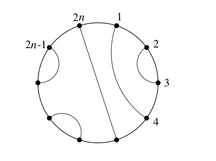Figure 5: An example of non-intersecting loops in a plane.

Consider a circle, with $2n$ points on its circumference. These points are connected by $n$ non-intersecting lines within the circle. Each point is connected to precisely one other point. See an example in the Figure 5.

The problem is now to derive the number of ways these $2n$ points can be pairwise connected. Obviously, for $n=1$ we have 2 points, which can only be connected to one another, so $c_1=1$. For $n=2$ one has 4 points, and $c_2=2$. Namely, point 1 can be connected to point 2 or to point 4. Connection of point 1 to point 3 is not allowed, because it intersects the line between points 2 and 4. The points are numbered clockwise. We use the notation $c_0=1$.

[1] 2 points Let there be a line connecting point 1 to point $2n$. The remaining points are divided into two groups by this line. On this basis, write down a recursion formula for $c_n$ for general $n$.

[2] 2 points Use the definition of the so-called generating function

$$P(x)=\sum _{k=0}^{\infty }{c}_k{x}^k$$

and the recursion found under part [1] to derive an equation that $P(x)$ must satisfy. Solve this equation, which yields $P(x)$ as an explicit function of $x$.

[3] 2 points Using this solution, obtain the first few terms in the Taylor expansion of $xP(x)={\sum }_k{a}_k{x}^k$. Derive the ratio $a_k/a_{k-1}$ for general $k$. Write the similar ratio $c_n/c_{n-1}$ as a function of $n$.

[4] 2 points Give $c_n$ as an explicit function of $n$.

[5] 2 points The corresponding contribution $\Delta S$ to the entropy of a system is $\Delta S=k_B\ln (c_n)$ where $k_B$ is Boltzmann’s constant. How does $\Delta S$, in leading order, depend on $n$ in the limit of large $n$?

Fonte: Testo (PDF) — p.14 Topic: Mathematics, Thermodynamics Metodi: Approximation & Series Expansion, Statistical Averaging, Physical Modeling Competenze: Mathematical Modeling, Physical Reasoning Objects: —

Connecting the dots Henk Blöte, Leiden University

Alcuni problemi bidimensionali nella fisica statistica, come un sistema di polimeri, e i modelli Ising, XY e Heisenberg, possono essere formulati in termini di somma su tutte le configurazioni di cicli non intersezionati in un piano. Nell’esame di questi modelli di loop si presenta il seguente problema.

Figura 5: Un esempio di cicli non incrociati in un piano.

Considerate un cerchio, con $2n$ punti sulla sua circonferenza. Questi punti sono collegati da linee non intersezionate $n$ all’interno del cerchio. Ogni punto è collegato a un altro punto. Vedi un esempio nella Figura 5.

Il problema è ora quello di derivare il numero di modi in cui questi punti $2n$ possono essere collegati in coppia. Ovviamente, per $n=1$ abbiamo 2 punti, che possono essere collegati tra loro, quindi $c_1=1$. Per $n=2$ si hanno 4 punti e $c_2=2$. Il punto 1 può essere collegato al punto 2 o al punto 4. Non è consentito collegare il punto 1 al punto 3, poiché interseca la linea tra i punti 2 e 4. I punti sono numerati in senso orario. Utilizziamo la notazione $c_0=1$.

[1] 2 punti Deve esserci una linea che collega il punto 1 al punto $2n$. I punti rimanenti sono divisi in due gruppi con questa linea. Su questa base, scrivere una formula di ricorrenza per $c_n$ per $n$ generale.

[2] 2 punti Utilizzare la definizione della cosiddetta funzione di generazione

$$P(x)=\sum _{k=0}^{\infty }{c}_k{x}^k$$

e la ricorsione trovata nella parte [1] per derivare un’equazione che $P(x)$ deve soddisfare. Risolvi questa equazione, che dà $P(x)$ come funzione esplicita di $x$.

[3] 2 punti Usando questa soluzione, ottenere i primi termini nell’espansione Taylor di $xP(x)={\sum }_k{a}_k{x}^k$. Derivare il rapporto $a_k/a_{k-1}$ per $k$ generale. Scrivere il rapporto simile $c_n/c_{n-1}$ come funzione di $n$.

[4] 2 punti Indicare $c_n$ come funzione esplicita di $n$.

[5] 2 punti Il corrispondente contributo $\Delta S$ all’entropia di un sistema è $\Delta S=k_B\ln (c_n)$ dove $k_B$ è la costante di Boltzmann. Come $\Delta S$, in ordine di primo piano, dipende da $n$ nel limite di grande $n$?

Fonte: Testo (PDF) — p.14 Topic: Mathematics, Thermodynamics Metodi: Approximation & Series Expansion, Statistical Averaging, Physical Modeling Competenze: Mathematical Modeling, Physical Reasoning Objects: —

Glaciers and climate change — Michiel Helsen, Utrecht University

As a consequence of climate fluctuations, glaciers vary in length. We can study the sensitivity of glaciers to climate change with a simple model.

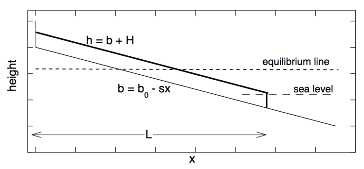Figure 6: A sketch of a glacier with constant slope.

Figure 6 considers a glacier with length $L$, constant thickness $H$ and flowing on a bed $b(x)$ with a small constant slope $s$: $b=b_0-sx$ with $x=0$ the top of the glacier. The height of the bed $h$ is expressed with respect to sea level. We assume that the glacier has a constant width. Water and ice density are denoted by ${\rho }_{\text{water}}$ and ${\rho }_{\text{ice}}$, respectively. When the glacier reaches the ocean, calving occurs as the ice reaches flotation, i.e. there is no floating ice tongue.

[1] 2 points Find the length of the part of the glacier extending into the ocean, note that $L$ is the glacier length in $x$-direction (not along the bed).

Besides floatation the calving rate at the glacier front is proportional to the water depth, which we write as: $c{b}_L$. Apart from ice loss at the calving front, the glacier gains or loses mass at its surface, which is called the Specific Mass Balance SMB. It is defined as the mass of ice that accumulates or is removed per year at a specific point on the glacier surface. As such, it is the resultant of many meteorological processes that determine the exchange of mass between atmosphere and glacier surface (snowfall, rime, melt, sublimation, etc). We assume that the specific balance varies as: $SMB(h)=\beta (h-E)$, where $h$ is the height above sea level, $\beta$ is the balance gradient (a constant) and $E$ is the equilibrium line altitude, which separates the accumulation area from the ablation area.

[2] 3 points Find the solution(s) for the equilibrium length of the glacier, as a function of $E$.

[3] 1 point Ice flows under the influence of gravity. Considering that the glacier geometry is in equilibrium, at which point do we find the highest ice velocity?

Assume for part [4] the simple case that the glacier terminus does not reach the ocean.

[4] 3 points The mean temperature of the atmosphere decreases with height. Assume that $E$ coincides with an isotherm in the atmosphere. Find an expression for the sensitivity of the glacier for a temperature change, i.e. $\frac{dL}{dT}$. The atmospheric temperature gradient is a constant $\gamma$.

[5] 1 point How does this sensitivity changes when temperatures drop and the glacier front reaches the ocean? Show this qualitatively in a sketch.

Fonte: Testo (PDF) — p.16 Topic: Earth & Environmental Science, Fluid Mechanics Metodi: Hydrostatic Equilibrium, Physical Modeling, Differential Equations Competenze: Mathematical Modeling, Physical Reasoning Objects: —

Glicieri e cambiamenti climatici Michiel Helsen, Università di Utrecht

A causa delle fluttuazioni climatiche, i ghiacciai variano di lunghezza. Possiamo studiare la sensibilità dei ghiacciai ai cambiamenti climatici con un modello semplice.

Figura 6: Sketta di un ghiacciaio con pendenza costante.

La figura 6 considera un ghiacciaio di lunghezza $L$, spessore costante $H$ e che scorre su un letto $b(x)$ con una piccola pendenza costante $s$: $b=b_0-sx$ con $x=0$ la parte superiore del ghiacciaio. L’altezza del letto $h$ è espressa rispetto al livello del mare. Supponiamo che il ghiacciaio abbia una larghezza costante. La densità dell’acqua e del ghiaccio sono indicati rispettivamente da ${\rho }_{\text{water}}$ e ${\rho }_{\text{ice}}$. Quando il ghiacciaio raggiunge l’oceano, il calvamento si verifica quando il ghiaccio raggiunge la flottazione, cioè Non c’è una lingua di ghiaccio galleggiante.

[1] 2 punti Trova la lunghezza della parte del ghiacciaio che si estende nell’oceano, nota che $L$ è la lunghezza del ghiacciaio nella direzione $x$ (non lungo il letto).

Oltre alla fluttuazione, la velocità di calvamento al fronte del ghiacciaio è proporzionale alla profondità dell’acqua, che scriviamo come: $c{b}_L$. Oltre alla perdita di ghiaccio al fronte di calvamento, il ghiacciaio guadagna o perde massa sulla sua superficie, che viene chiamata SMB di bilanci di massa specifici. Si definisce come la massa di ghiaccio che si accumula o si rimuove ogni anno in un punto specifico sulla superficie del ghiacciaio. Come tale, è il risultato di molti processi meteorologici che determinano lo scambio di massa tra l’atmosfera e la superficie dei ghiacciai (neve caduta, rime, fusione, sublimazione, ecc.). Supponiamo che il saldo specifico varia come: $SMB(h)=\beta (h-E)$, dove $h$ è l’altezza sopra il livello del mare, $\beta$ è il gradiente di equilibrio (una costante) e $E$ è l’altitudine della linea di equilibrio, che separa la superficie di accumulazione dalla superficie di ablazione.

[2] 3 punti Trova la soluzione(s) per la lunghezza di equilibrio del ghiacciaio, come funzione di $E$.

[3] 1 punto I ghiacci fluiscono sotto l’influenza della gravità. Considerando che la geometria del ghiacciaio è in equilibrio, a quale punto troviamo la velocità di ghiaccio più alta?

Supponiamo per parte [4] il caso semplice che il terminale del ghiacciaio non raggiunga l’oceano.

**[4] ** 3 punti La temperatura media dell’atmosfera diminuisce con l’altezza. Supponiamo che $E$ coincida con un isotermo nell’atmosfera. Trovare un’espressione per la sensibilità del ghiacciaio a un cambiamento di temperatura, cioè $\frac{dL}{dT}$. Il gradiente di temperatura atmosferica è costante $\gamma$.

Come cambia questa sensibilità quando le temperature scendono e il fronte del ghiacciaio raggiunge l’oceano? Mostra questo in modo qualitativo in uno sketch.

Fonte: Testo (PDF) — p.16 Topic: Earth & Environmental Science, Fluid Mechanics Metodi: Hydrostatic Equilibrium, Physical Modeling, Differential Equations Competenze: Mathematical Modeling, Physical Reasoning Objects: —

24 Hours in a Day – are there? — Gerhard Blab, Utrecht University

We all know that there are 24 hours in a day. If we look more closely, it turns out, this is not quite correct: a true solar day in late December is up to half a minute longer than the expected 24 hours, while in mid-September we are all shortchanged 20 seconds! Only averaged over a year, a “mean” solar day measures the regulation 24 hours.

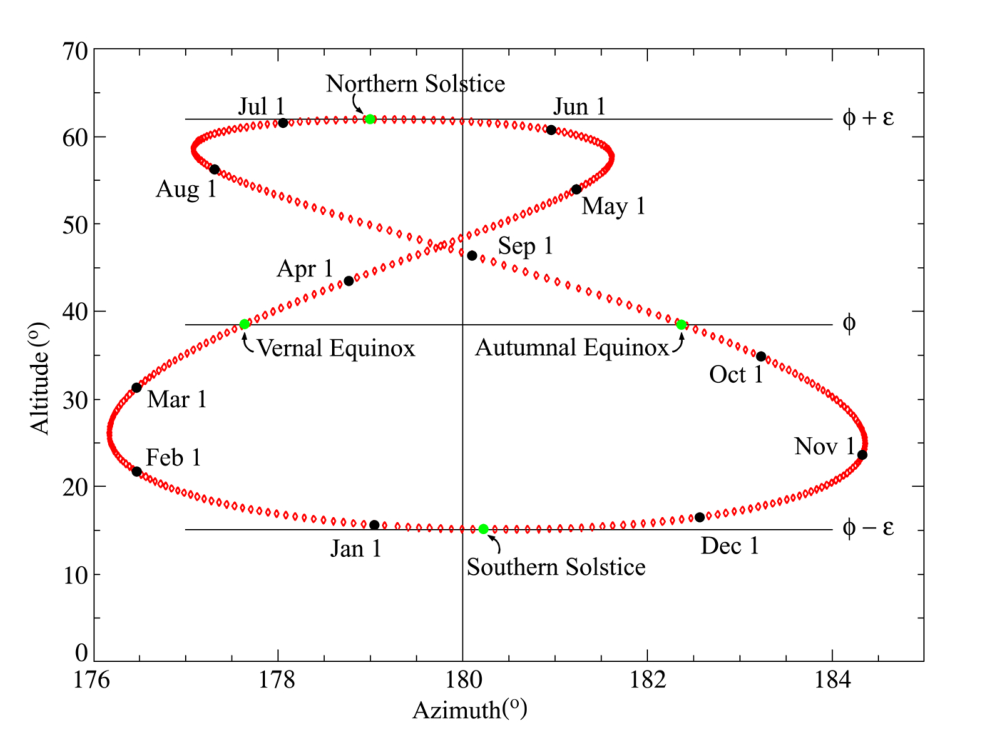Figure 7: Position of the sun at 12:00 noon GMT as seen at the Royal Observatory, Greenwich, UK (lat $51.5^{\circ }$N, long $0^{\circ }$W); Earth’s last perihelion (147 Gm) occurred on January 4th, 2014, and its next aphelion (152 Gm) will be on July 4th.

To tackle this problem, I need to tell you what I mean by a “true” solar day: it is the time between two local noons, that is times at which your shadow will point exactly north (or south, if you are in Australia).

[1] 3 points Argue and sketch how the orbital motion of Earth around the sun leads to a mean solar day that is longer than the rotation of the Earth, and show that this difference should indeed be on the order of 4 minutes. Make sure to clearly indicate directions of rotation!

[2] 3 points Figure 7 shows an “Analemma”, a figure obtained by plotting the position of the sun every 24 hours over the course of a year. In it you can find back the seasonal change of altitude, as well as offset between our 24 hour “mean solar day” and the true solar time. Use the figure to estimate the four times during a year at which a day is actually close to 24 hours long, and plot the offset as a function of date (y axis: offset in minutes; x axis: months). This representation is also called the “equation of time”.

[3] 4 points The equation of time is caused by two different effects, both comparable in magnitude: the eccentricity of Earth’s orbit and the obliquity (“tilt”) of its axis. Explain how those two effects influence the length of a true solar day during a year, and sketch their independent contributions to the equation of time.

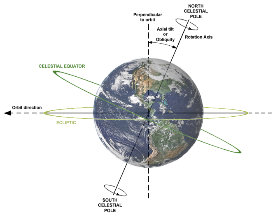Figure 8: Axis Tilt (Obliquity) of Earth.

Fonte: Testo (PDF) — p.18 Topic: Astrophysics, Gravitation Metodi: Kepler’s Laws, Physical Modeling, Order-of-Magnitude Estimation Competenze: Diagrammatic Reasoning, Physical Reasoning Objects: Planet, Star

24 ore al giorno sono presenti? * Gerhard Blab, Università di Utrecht*

Sappiamo tutti che ci sono 24 ore al giorno. Se si guarda più da vicino, si scopre che non è proprio così: un vero giorno solare alla fine di dicembre è fino a mezzo minuto più lungo delle 24 ore previste, mentre a metà settembre ci mancano tutti 20 secondi! Solo una giornata solare “media” misura la regolazione di 24 ore.

Figura 7: posizione del sole alle 12:00 mezzogiorno GMT osservata presso l’Osservatorio Reale di Greenwich, Regno Unito (lat $51.5^{\circ }$N, lungo $0^{\circ }$W); l’ultimo perihelione della Terra (147 Gm) si è verificato il 4 gennaio 2014, e il suo prossimo aphelione (152 Gm) sarà il 4 luglio.

Per affrontare questo problema, devo dirvi cosa intendo con un “vero” giorno solare: è l’ora tra due mezzogiorno locali, cioè i momenti in cui la vostra ombra punta esattamente a nord (o a sud, se siete in Australia).

[1] 3 punti Argomenti e schizzi di come il movimento orbitale della Terra attorno al Sole porta a un giorno solare medio che è più lungo della rotazione della Terra, e mostrare che questa differenza dovrebbe effettivamente essere nell’ordine di 4 minuti. Assicurati di indicare chiaramente le direzioni di rotazione!

[2] 3 punti La figura 7 mostra un “Analemma”, una cifra ottenuta tracciando la posizione del sole ogni 24 ore nel corso di un anno. In esso si può ritrovare il cambiamento stagionale dell’altitudine, così come la compensazione tra la nostra “giornata solare media” di 24 ore e l’ora solare vera. Utilizzare la figura per stimare le quattro volte in un anno in cui un giorno è effettivamente di circa 24 ore di lunghezza e tracciare il compensazione in funzione della data (asse y: compensazione in minuti; asse x: mesi). Questa rappresentazione è anche chiamata “equazione del tempo”.

[3] 4 punti L’equazione del tempo è causata da due effetti diversi, entrambi comparabili in magnitudine: l’escentricità dell’orbita terrestre e l’inclinazione (“inclinazione”) del suo asse. Spiegate come questi due effetti influenzino la durata di un vero giorno solare durante un anno e descrivete il loro contributo indipendente all’equazione del tempo.

Figura 8: Tilt dell’asse (Obliquità) della Terra.

Fonte: Testo (PDF) — p.18 Topic: Astrophysics, Gravitation Metodi: Kepler’s Laws, Physical Modeling, Order-of-Magnitude Estimation Competenze: Diagrammatic Reasoning, Physical Reasoning Objects: Planet, Star

Dzyaloshinskii-Moriya interactions and skyrmions — Rembert Duine, Utrecht University

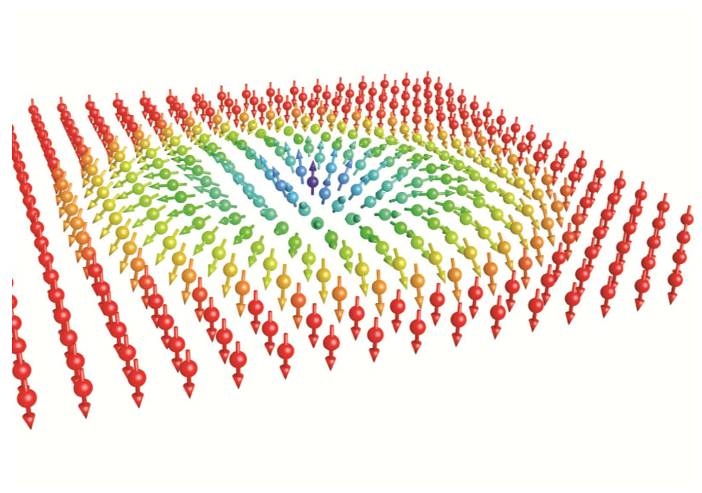Figure 9: Example of a magnetic skyrmion. The magnetization points up at the skyrmion core and down away from the core.

A ferromagnetic material far below its critical temperature is characterized by a direction of magnetization $\mathbf{m}(\mathbf{x})$ (a unit vector) that can, in general, be a function of the three-dimensional position $\mathbf{x}$. For ordinary ferromagnets, the energy is given by

$$E[\mathbf{m}]=\int d\mathbf{x}\left[-\frac{J}{2}\mathbf{m}(\mathbf{x})\cdot {\nabla }^2\mathbf{m}(\mathbf{x})\right]$$

where $J>0$ is the so-called spin stiffness.

[1] 2 points Give the configuration of $\mathbf{m}(\mathbf{x})$ with the lowest energy.

In certain ferromagnets (to be more precise, in ferromagnets without inversion symmetry) there are additional terms in the energy, called Dzyaloshinskii-Moriya interactions. One possibility is a term of the form $\mathbf{m}\cdot \nabla \times \mathbf{m}$, so that the energy now reads

$$E[\mathbf{m}]=\int d\mathbf{x}\left[-\frac{J}{2}\mathbf{m}(\mathbf{x})\cdot {\nabla }^2\mathbf{m}(\mathbf{x})+\frac{D}{2}\mathbf{m}(\mathbf{x})\cdot (\nabla \times \mathbf{m}(\mathbf{x}))\right]$$

with $D>0$ a constant.

[2] 2 points Derive the Euler-Lagrange equations for $\mathbf{m}(\mathbf{x})$ by minimizing this energy functional, and show that you obtain

$$J{\nabla }^2\mathbf{m}(\mathbf{x})=D\nabla \times \mathbf{m}(\mathbf{x})$$

Show that a possible solution of this equation is a so-called spin spiral:

$$\mathbf{m}(\mathbf{x})=\cos (qx)\hat{y}+\sin (qx)\hat{z}$$

and determine $q$.

Other examples of low-energy configurations are so-called skyrmions (see Figure 9) for which the magnetization depends only on the coordinates in the $x-y-$plane, i.e., $\mathbf{m}(\mathbf{x})=\mathbf{m}(x,y)$. Skyrmions correspond to excitations where the magnetization is up (or down) at a certain position (the position of the skyrmion), whereas it is down (or up) away from this position. For skyrmions the so-called winding number $W$ is equal to $+1$ (or $-1$ for anti-skyrmions). This winding number is defined by

$$W=\int \frac{dxdy}{(4\pi )}\mathbf{m}\cdot \left(\frac{\partial \mathbf{m}}{\partial x}\times \frac{\partial \mathbf{m}}{\partial y}\right)$$

[3] 3 points Show that this winding number is an integer. (This means that smooth evolutions of the magnetization cannot lead to changes in the winding number, so that skyrmions are what is called “topologically protected”).

Hint: one approach is to parameterize the unit vector $\mathbf{m}$ in terms of angles $\theta (\rho ,\varphi )$ and $\phi (\rho ,\varphi )$ according to $\mathbf{m}=(\sin (\theta )\cos (\phi ),\sin (\theta )\sin (\phi ),\cos (\theta ))$. These angles depend polar coordinates $(\rho ,\varphi )$ in the plane. Rewrite the winding number in terms of $\rho$ and $\varphi$. Evaluate this for skyrmions for which $\rho$ depends on $\varphi$ only.

A possible ansatz for the description of a skyrmion is to assume

$$\mathbf{m}=\sin \theta (\rho )\hat{\rho }+\cos \theta (\rho )\hat{z}$$

where $(\rho ,\varphi ,z)$ are cylindrical coordinates.

[4] 3 points Derive the equation of motion for $\theta (\rho )$, starting from the energy that includes a field in the $z$-direction, i.e., starting from

$$E[\mathbf{m}]=\int d\mathbf{x}\left[-\frac{J}{2}\mathbf{m}(\mathbf{x})\cdot {\nabla }^2\mathbf{m}(\mathbf{x})+\frac{D}{2}\mathbf{m}(\mathbf{x})\cdot (\nabla \times \mathbf{m}(\mathbf{x}))-B\mathbf{m}(\mathbf{x})\cdot \hat{z}\right]$$

where $B$ is the magnitude of the field in appropriate units.

You might find the cylindrical Laplacian useful

$${\nabla }^2=\frac{{\partial }^{2}f}{\partial r^2}+\frac{1}{r}\frac{\partial f}{\partial r}+\frac{1}{r^2}\frac{{\partial }^{2}f}{\partial {\theta }^2}+\frac{{\partial }^{2}f}{\partial z^2}$$

Fonte: Testo (PDF) — p.20 Topic: Magnetism, Modern-Quantum Physics Metodi: Differential Equations, Calculus-Integration, Energy Conservation Method, Symmetry Argument Competenze: Mathematical Modeling, Physical Reasoning Objects: —

Interazioni di Dzyaloshinskii-Moriya e skyrmioni — Rembert Duine, Utrecht University

Figure 9: Example of a magnetic skyrmion. The magnetization points up at the skyrmion core and down away from the core.

Un materiale ferromagnetico ben al di sotto della sua temperatura critica è caratterizzato da una direzione di magnetizzazione $\mathbf{m}(\mathbf{x})$ (un versore) che può, in generale, essere funzione della posizione tridimensionale $\mathbf{x}$. Per i ferromagneti ordinari, l’energia è data da

$$E[\mathbf{m}]=\int d\mathbf{x}\left[-\frac{J}{2}\mathbf{m}(\mathbf{x})\cdot {\nabla }^2\mathbf{m}(\mathbf{x})\right]$$

dove $J>0$ è la cosiddetta rigidità di spin.

[1] 2 punti Fornisci la configurazione di $\mathbf{m}(\mathbf{x})$ con l’energia più bassa.

In certi ferromagneti (più precisamente, nei ferromagneti privi di simmetria di inversione) ci sono termini aggiuntivi nell’energia, chiamati interazioni di Dzyaloshinskii-Moriya. Una possibilità è un termine della forma $\mathbf{m}\cdot \nabla \times \mathbf{m}$, cosicché l’energia diventa

$$E[\mathbf{m}]=\int d\mathbf{x}\left[-\frac{J}{2}\mathbf{m}(\mathbf{x})\cdot {\nabla }^2\mathbf{m}(\mathbf{x})+\frac{D}{2}\mathbf{m}(\mathbf{x})\cdot (\nabla \times \mathbf{m}(\mathbf{x}))\right]$$

con $D>0$ una costante.

[2] 2 punti Ricava le equazioni di Euler-Lagrange per $\mathbf{m}(\mathbf{x})$ minimizzando questo funzionale dell’energia, e mostra che si ottiene

$$J{\nabla }^2\mathbf{m}(\mathbf{x})=D\nabla \times \mathbf{m}(\mathbf{x})$$

Mostra che una possibile soluzione di questa equazione è una cosiddetta spirale di spin:

$$\mathbf{m}(\mathbf{x})=\cos (qx)\hat{y}+\sin (qx)\hat{z}$$

e determina $q$.

Altri esempi di configurazioni a bassa energia sono i cosiddetti skyrmioni (vedi Figura 9) per i quali la magnetizzazione dipende solo dalle coordinate nel $x-y-$piano, cioè $\mathbf{m}(\mathbf{x})=\mathbf{m}(x,y)$. Gli skyrmioni corrispondono a eccitazioni in cui la magnetizzazione è verso l’alto (o verso il basso) in una certa posizione (la posizione dello skyrmione), mentre è verso il basso (o verso l’alto) lontano da questa posizione. Per gli skyrmioni il cosiddetto numero di avvolgimento $W$ è uguale a $+1$ (oppure $-1$ per gli anti-skyrmioni). Questo numero di avvolgimento è definito da

$$W=\int \frac{dxdy}{(4\pi )}\mathbf{m}\cdot \left(\frac{\partial \mathbf{m}}{\partial x}\times \frac{\partial \mathbf{m}}{\partial y}\right)$$

[3] 3 punti Mostra che questo numero di avvolgimento è un intero. (Ciò significa che evoluzioni regolari della magnetizzazione non possono portare a variazioni del numero di avvolgimento, cosicché gli skyrmioni sono ciò che viene chiamato “topologicamente protetto”).

Suggerimento: un approccio consiste nel parametrizzare il versore $\mathbf{m}$ in termini degli angoli $\theta (\rho ,\varphi )$ e $\phi (\rho ,\varphi )$ secondo $\mathbf{m}=(\sin (\theta )\cos (\phi ),\sin (\theta )\sin (\phi ),\cos (\theta ))$. Questi angoli dipendono dalle coordinate polari $(\rho ,\varphi )$ nel piano. Riscrivi il numero di avvolgimento in termini di $\rho$ e $\varphi$. Valutalo per gli skyrmioni per i quali $\rho$ dipende solo da $\varphi$.

Un possibile ansatz per la descrizione di uno skyrmione è assumere

$$\mathbf{m}=\sin \theta (\rho )\hat{\rho }+\cos \theta (\rho )\hat{z}$$

dove $(\rho ,\varphi ,z)$ sono coordinate cilindriche.

[4] 3 punti Ricava l’equazione del moto per $\theta (\rho )$, partendo dall’energia che include un campo nella direzione $z$, cioè partendo da

$$E[\mathbf{m}]=\int d\mathbf{x}\left[-\frac{J}{2}\mathbf{m}(\mathbf{x})\cdot {\nabla }^2\mathbf{m}(\mathbf{x})+\frac{D}{2}\mathbf{m}(\mathbf{x})\cdot (\nabla \times \mathbf{m}(\mathbf{x}))-B\mathbf{m}(\mathbf{x})\cdot \hat{z}\right]$$

dove $B$ è il modulo del campo in unità appropriate.

Potrebbe esserti utile il laplaciano cilindrico

$${\nabla }^2=\frac{{\partial }^{2}f}{\partial r^2}+\frac{1}{r}\frac{\partial f}{\partial r}+\frac{1}{r^2}\frac{{\partial }^{2}f}{\partial {\theta }^2}+\frac{{\partial }^{2}f}{\partial z^2}$$

Fonte: Testo (PDF) — p.20 Topic: Magnetism, Modern-Quantum Physics Metodi: Differential Equations, Calculus-Integration, Energy Conservation Method, Symmetry Argument Competenze: Mathematical Modeling, Physical Reasoning Objects: —