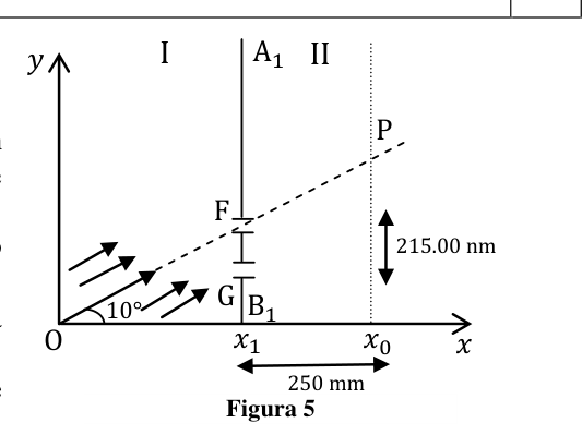
Figura 5
Pag. 1 di 2 T-2 Q
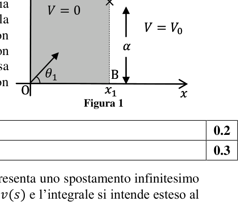
Il Principio Variazionale (Punteggio Totale: 10) A Il Principio Variazionale in Meccanica Considera il piano orizzontale x-y privo di attrito della Fig. 1. È diviso in due regioni, I and II, da una linea AB di equazione . L’energia potenziale di una particella puntiforme di massa è nella regione I, mentre è nella regione II. La particella è lanciata con velocità dall’origine O, in una direzione che forma l’angolo con l’asse x. Essa raggiunge un punto P nella regione II, viaggiando in essa con una velocità secondo una direzione che forma l’angolo con l’asse x. In tutto T-2 (in tutte le parti del problema) trascura la gravità e gli effetti relativistici.
A1 Ricava un’espressione di in funzione di , e . 0.2 A2 Esprimi in funzione di , e . 0.3
Si definisce una grandezza , chiamata azione; rappresenta uno spostamento infinitesimo lungo la traiettoria per una particella di massa , in moto con velocità e l’integrale si intende esteso al cammino. Per esempio, nel caso di una particella in moto lungo un percorso circolare di raggio , con velocità di modulo costante , l’azione per un giro è . Per una particella di energia costante , si può dimostrare che, fra tutte le possibili traiettorie tra due punti dati, la traiettoria effettiva è quella in cui la grandezza definita sopra assume un valore estremo (minimo oppure massimo). Storicamente, questo caso è noto come Principio di Minima Azione (PMA).
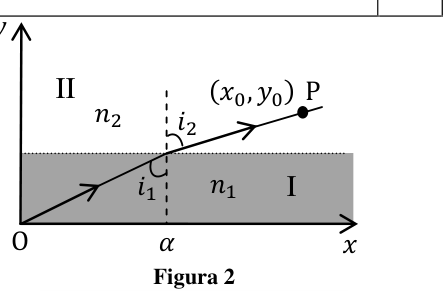
A3 Dal PMA si deduce che la traiettoria di una particella in moto tra due punti dati in una regione con potenziale costante deve essere rettilinea. Supponiamo che i due punti fissi e della Fig. 1 abbiano rispettivamente coordinate e ; il punto di confine nel quale la particella passa dalla regione I alla regione II abbia coordinate Osserva che è fisso e che l’azione dipende soltanto dalla coordinata . Ricava l’espressione dell’azione . Usa il PMA per ricavare la relazione tra e queste coordinate. 1.0 B Il Principio Variazionale in Ottica Un raggio di luce passa da un mezzo I a un mezzo II con indici di rifrazione rispettivamente e . I due mezzi sono separati da una linea parallela all’asse x. Il raggio di luce forma un angolo con l’asse y nel mezzo I e un angolo nel mezzo II (vedi Fig. 2). Per ottenere la traiettoria del raggio, faremo uso di un altro principio variazionale (di minimo o massimo), noto come principio di Fermat del tempo minimo.
B1 Il principio stabilisce che, tra due punti dati, un raggio luminoso si muove lungo un cammino tale che il tempo impiegato tra i due punti risulti un estremo. In base al principio di Fermat, ricava la relazione tra e . 0.5
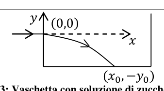
Nella Fig. 3 è disegnato schematicamente il percorso di un raggio laser che incide orizzontalmente su una soluzione di zucchero, nella quale la concentrazione dello zucchero decresce con l’altezza. Di conseguenza, anche l’indice di rifrazione della soluzione decresce con l’altezza.
B2 Supponi che l’indice di rifrazione dipenda soltanto da . Usa l’equazione ottenuta in B1 per ricavare l’espressione della pendenza del cammino del raggio in funzione dell’indice di rifrazione , corrispondente a , e di . 1.5 B3 Il fascio laser parte dall’origine in direzione orizzontale ed entra nella soluzione zuccherina a un’altezza dal fondo della vaschetta, come si vede nella figura 3. Poni , dove e sono costanti positive. Per la traiettoria effettiva del fascio laser, ricava un’espressione di in funzione di 1.2 Figura 2 Figura 1 Figura 3: Vaschetta con soluzione di zucchero
I II
Pag. 2 di 2 T-2 Q e delle grandezze associate. Puoi usare la relazione: costante, dove ⁄
oppure la relazione:
( ) B4 Ricava il valore di , il punto in cui il fascio luminoso tocca il fondo della vaschetta. Poni cm, , cm (1 cm = 10-2 m). 0.8
C Il Principio Variazionale e la Natura Ondulatoria della Materia Esploreremo ora il rapporto tra il PMA e la natura ondulatoria di una particella in moto. A questo scopo, ammettiamo che una particella che si muova a possa percorrere tutte le possibili traiettorie e cerchiamo una traiettoria che sia il risultato dall’interferenza costruttiva tra le onde di de Broglie.
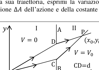
C1 Posto che una particella descriva un tratto infinitesimale della sua traiettoria, esprimi la variazione della fase della sua onda di de Broglie in funzione della variazione dell’azione e della costante di Planck. 0.6 C2 Riprendi il problema della Parte A in cui la particella passa da a (vedi Fig. 4). Supponiamo di porre una separazione opaca al confine tra le due regioni. In è presente una piccola apertura , di larghezza , tale che e .
Considera due cammini estremi e , in modo che giaccia sulla traiettoria classica discussa nella parte A. Ricava la differenza di fase tra i due cammini, al primo ordine di approssimazione. 1.2 D Interferenza delle Onde Materiali Considera un cannone elettronico collocato in , che invia un fascio collimato di elettroni su una stretta fenditura ; questa è ricavata nella separazione opaca in una posizione così che risulti un percorso rettilineo. è un punto sullo schermo in (vedi Fig. 5). La velocità in I è m s e si ha . Il potenziale in II è tale che la velocità risulti m s . La distanza è di ( ). Trascura l’interazione elettrone-elettrone.
D1 Supponendo che gli elettroni in siano stati accelerati da fermi, calcola il potenziale acceleratore . 0.3 D2 Nella separazione si ricava una seconda fenditura identica a una distanza di nm ( nm m) al di sotto della fenditura (Fig. 5). Indicando con la differenza di fase tra le onde di de Broglie che arrivano nel punto P attraverso le due fenditure F e G, calcola . 0.8 D3 Qual è la minima distanza da P per la quale ci si attende di trovare un valore nullo (zero) nella rivelazione degli elettroni sullo schermo? [Nota: può risultarti utile l’approssimazione ]. 1.2 D4 Il fascio ha una sezione trasversale quadrata di e l’apparato ha una lunghezza di 2 m. Quale deve essere la minima densità di flusso Imin (numero di elettroni per unità di area normale e per unità di tempo) affinché in qualunque istante si abbia, in media, almeno un elettrone nell’apparato? 0.4
Figura 4 Figura 5
215.00 nm
250 mm
p.1 — Piano con regioni I e II, traiettoria
p.1 — Rifrazione tra mezzi n1 e n2
p.1 — Vaschetta con soluzione di zucchero
p.2 — Traiettorie A,B,C,D tra regioni
p.2 — Fronti d’onda inclinati, punti F G
Topic: Modern-Quantum Physics, Geometric Optics, Newtonian Mechanics Metodi: de Broglie Relation, Snell’s Law, Differential Equations, Conservation of Energy, Interference & Diffraction Analysis, Small-Angle Approximation Competenze: Mathematical Modeling, Physical Reasoning, Diagrammatic Reasoning Objects: Slit, Screen, Electron Fonte: Testo (PDF) — p.1 Soluzione: Soluzioni (PDF)
The following table shows the results of the calculation of the total cost of the vehicle:
Pay it. 1 di 2 T-2 Q
The Principle of Variation (Scoring) Total: 10 The Principle of Variability in Mechanics Consider the friction-free x-y horizontal plane of the Fig. 1. It is divided into Two regions, I and II, from a line AB of the equation. Energy The potential of a pointed particle mass is in The Commission has already decided to adopt a proposal for a regulation on the approximation of the laws of the Member States relating to the use of the electricity sector in the Community. The particle was launched with speed from the origin O, in a direction that forms the angle with The x-axis. It reaches a point P in Region II, travelling through it with a velocity in a direction that forms the angle with The x-axis. All in all T-2 (in all parts of the problem) neglects gravity And the relativistic effects.
A1 It takes an expression of function of , and . 0.2 A2 Expressions in terms of , e . 0.3
A size is defined, called action; it represents an infinitesimal displacement The trajectory of a moving mass particle along a velocity and integral path is extended to the I’m going to walk. For example, in the case of a moving particle along a circular path of radius, with The action for a spin is . For a particle of constant energy , yes . It can demonstrate that, between all possible trajectories between two data points, the actual trajectory is that where the The size defined above takes on an extreme value (minimum or maximum). Historically, this case is known as the Minimum Action Principle (MAP).
A3 The MPA shows that the trajectory of a moving particle between two data points in a region with The constant potential must be straight. Let’s say the two fixed points and Fig. 1 have coordinates and ; the border point where the particle passes through Region I respectively The Commission has a number of proposals for a new programme for the European Community. Coordinated . It was the expression of action . Use the WFP to obtain the relationship between These coordinates. 1.0 B The principle of variation in optics A beam of light passes from a medium I to a medium II with indices of refraction and . The two means are separated by a line parallel to the x-axis. The light beam forms an angle with the y-axis in the The average of the two samples is the average of the two samples. 2). In order to obtain the The radius trajectory, we will use another variational principle (of The maximum or minimum time) known as the Fermat principle of minimum time.
B1 The principle states that between two data points a beam of light moves along a path such that the The time taken between the two points is extreme. The Fermat principle states that the relationship between the two e . 0.5
In the Fig. 3 is the path of a laser beam diagrammed The sugar content of the product is not to exceed the limit of the quantity of sugar in the product. The concentration of sugar decreases with height. As a result, The refractive index of the solution decreases with height.
B2 Suppose the refractive index depends only on . Use the equation obtained in B1 to obtain The slope of the radius path is expressed as a function of the refractive index , corresponding to , and of . 1.5 B3 The laser beam starts from the source in a horizontal direction and enters the sugar solution in the a height from the bottom of the tank, as shown in Figure 3. Pons , where and They’re constantly positive. For the actual trajectory of the laser beam, it is expressed as a function of 1.2 Figure 2 The following is the list of the following: Figure 3: Baskets with sugar solution
I II
Pay it. 2 di 2 T-2 Q and the associated greatness. You can use the ratio: constant, where ⁄
or the report:
( ) B4 It takes the value of , the point where the light beam touches the bottom of the tank. Put your cm, , cm (1 cm = 10-2 m). 0.8
C The Principle of Variation and the Wave Nature of Matter We will now explore the relationship between the PMA and the wave nature of a moving particle. For that purpose, Let’s say that a particle that moves to can travel all the possible paths and we look for A trajectory that is the result of constructive interference between de Broglie waves.
C1 Since a particle describes an infinitesimal stretch of its trajectory, it expresses the variation The resulting waveform is the de Broglie wave phase, which is a function of the change in the action and the constant of the Planck, please. 0.6 C2 Take the problem of Part A where the particle goes from a to a (see Fig. 4). Suppose we put a blurry separation on the The border between the two regions. In this case, a small Open , wide , as it is .
Consider two extreme paths and , so that The classical trajectory described in Part A. He was getting the The first step is the phase difference between the two paths, in the first order of The approximation is 1.2 D Interference of material waves Consider an electronic cannon placed in , which sends a a beam of electrons collimated on a narrow crack; this is obtained from opaque separation in a position So it’s a straight path. It’s a point on the top. The screen in (see Fig. 5). The velocity in I is m s e si ha . The potential in II is such that the The speed of the result m s . The distance è di ( ). Interaction is traced The electron-electron.
D1 Assuming the electrons in were accelerated by stops, calculate the potential accelerator. 0.3 D2 In the separation a second split is made identical to a distance of nm (nm) (m) below the cleft (Fig. 5). Indicating by the phase difference between the waves of de Brokers coming to point P through the two fissures F and G, calculate. 0.8 D3 What is the minimum distance from P for which a zero value (zero) is expected to be found in the electron detection on the screen? [Note: approximation may be useful for you ]. 1.2 D4 The beam has a square cross section of and the apparatus has a length of 2 m. What is the minimum Imin flow density (number of electrons per unit of normal area and per unit of The time required for the device to be in operation is the time required for the device to be in operation. 0.4
Figure 4 Figure 5
215.00 nm
250 mm
Plan with regions I and II, trajectory
**p.1 ** Refraction between means n1 and n2
**p.1 ** Baskets with sugar solution
The Commission has also adopted a proposal for a Regulation (EC) laying down the rules for the implementation of the Community’s common fisheries policy.
The following shall be added to the list of the following:
Topic: Modern-Quantum Physics, Geometric Optics, Newtonian Mechanics Metodi: de Broglie Relation, Snell’s Law, Differential Equations, Conservation of Energy, Interference & Diffraction Analysis, Small-Angle Approximation Competenze: Mathematical Modeling, Physical Reasoning, Diagrammatic Reasoning Objects: Slit, Screen, Electron Fonte: Testo (PDF) — p.1 Soluzione: Soluzioni (PDF)