WoPhO 2012

Electrostatic Balloon — Deadline March 31, 2012

In this question we will investigate various aspects of a hypothetical aerostatic flying machine which we shall call electrostatic balloon. The idea is to take some electrically conducting metal foil and shape it into a sphere of radius $R$ (consider the foil to be essentially weightless and possess sufficient structural strength). Then evacuate it completely and, in order to balance the atmospheric pressure, charge the balloon by a suitable electrostatic charge $Q$. The buoyant force will arise from Archimedes’ principle just as it happens with a conventional hot-air balloon, and the machine will be able to carry a payload of mass $M$.

Problems

To obtain full marks, give a succinct reasoning for your answers.

1. For a balloon of radius $R$ and total charge $Q$, find

• (a) the surface charge $\sigma$,
• (b) the electric field $\mathbf{E}(r)$ in all space,
• (c) the potential $V$ with respect to infinity,
• (d) the energy $W$ required to charge the sphere.

Take the permittivity of the surrounding air to be unity.

2. Find what surface charge $\sigma$ will exactly counter-balance the atmospheric pressure $P$. You may proceed as follows:

• (a) Consider a small patch on a general charged conducting surface. Show that the effective electric field which acts on the patch is ${\mathbf{E}}_{\text{effective}}=\frac{1}{2}({\mathbf{E}}_{+}+{\mathbf{E}}_{-})$ where ${\mathbf{E}}_{+}$ and ${\mathbf{E}}_{-}$ are the electric fields immediately above and below the conducting surface, respectively. (Hint: treat separately the electric field produced by the small patch and that produced by all other charges.)
• (b) Find what $\sigma$ is required so that the expanding electrostatic force balances the contracting atmospheric pressure.

3. We will now take into account that air has a small but non-zero conductivity $s$ (the inverse of resistivity $\rho =1/s$), which causes the balloon to discharge over time.

• (a) If the balloon is initially charged with $Q_0$ and left unattended, find how its charge will evolve with time $Q=Q(t)$.
• (b) Suppose we install a charger which compensates the discharge due to air and keeps the charge constant at $Q_0$. How much power $\Pi$ will it consume? Express it as a function of the balloon radius $R$ only.

4. The whole purpose of the balloon is to carry a payload of mass $M$ (in this problem neglect the mass of the balloon itself). Find how the following quantities depend on $M$:

• (a) total charge $Q$,
• (b) energy $W$ [refer to Problem 1.(d)],
• (c) power $\Pi$ [Problem 3.(b)].

5. Consider a conventional hot-air balloon. Assume it to be spherical. A gas burner heats up the air, so that its density decreases inside the balloon and Archimedes force provides buoyancy. Use physical reasoning and practical considerations to estimate how the required burner’s power depends on the payload of mass $M$. Assume the volume of mass $M$ does not contribute to the buoyant force. Comment on which kind of technology is better suited for flying. Any sound answer will be given credit.

6. In practice one can expect the electrostatic balloon to be not perfectly hermetic. Consequently, the vacuum inside will be slowly filled with air from the atmosphere. We can model the situation by imagining that in the balloon there are tiny holes with a total surface area $S\ll R^2$. Assume the volume of mass $M$ does not contribute to the buoyant force.

• (a) Let the atmospheric pressure be $P_1$ and the pressure inside the balloon $P_2\ll P_1$. Find the velocity of the gas $v_2$ when it enters the balloon through some tiny hole on the surface. Temperature of the atmosphere is $T_1$, adiabatic index $\gamma$, molar mass $\mu$. [Hints: Make use of the Bernoulli equation (conservation of energy for a fluid element). Assume that the gas flows fast enough so that it does not have time to exchange any heat with the surroundings.]
• (b) We install a pump which keeps the balloon pressure at $P_2\ll P_1$. Find the power consumed by such a pump and express it as a function of payload $M$. Assume the pump’s hole size is equal to $S$, and $P_2=0$.

Fonte: Testo (PDF) — p.1 Topic: Electrostatics, Fluid Mechanics Metodi: Gauss’s Law, Electric Potential Method, Bernoulli’s Equation, Hydrostatic Equilibrium Competenze: Physical Reasoning, Mathematical Modeling Objects: Conducting Sphere

Ballone elettrostatico Data limite 31 marzo 2012

In this question we will investigate various aspects of a hypothetical aerostatic flying machine which we shall call electrostatic balloon. L’idea è quella di prendere una pellicola metallica elettricamente conduttiva e di formarla in una sfera di raggio $R$ (considerare che la pellicola sia essenzialmente senza peso e posseda una resistenza strutturale sufficiente). Quindi evacuare completamente e, per bilanciare la pressione atmosferica, caricare il palloncino con una carica elettrostatica appropriata $Q$. La forza galleggiante deriverà dal principio di Archimede, come avviene con un normale pallone a aria calda, e la macchina sarà in grado di trasportare un carico utile di massa $M$.

Problemi

Per ottenere i voti completi, fornire un ragionamento conciso delle risposte.

1. Per un palloncino di raggio $R$ e carica totale $Q$, trovare

• a) la carica superficiale $\sigma$,
• b) il campo elettrico $\mathbf{E}(r)$ in tutto lo spazio,
• (c) il potenziale $V$ rispetto all’infinito,
• d) l’energia $W$ necessaria per caricare la sfera.

Prendi la permisione dell’aria circostante per essere unita’.

**2. ** Trova quale carica superficiale $\sigma$ controbilancerà esattamente la pressione atmosferica $P$. Potete procedere come segue:

• (a) Considerare un piccolo contratto su una superficie conduttiva generalmente carica. Mostra che il campo elettrico effettivo che agisce sul patch è ${\mathbf{E}}_{\text{effective}}=\frac{1}{2}({\mathbf{E}}_{+}+{\mathbf{E}}_{-})$ dove ${\mathbf{E}}_{+}$ e ${\mathbf{E}}_{-}$ sono i campi elettrici immediatamente sopra e sotto la superficie conduttrice, rispettivamente. (Signore: trattare separatamente il campo elettrico prodotto dalla piccola lamina e quello prodotto da tutte le altre cariche.)
• (b) Trova il $\sigma$ necessario affinché la forza elettrostatica in espansione bilanci la pressione atmosferica in contrazione.

3. Si terrà conto che l’aria ha una conductività piccola ma non zero $s$ (l’inverso della resistività $\rho =1/s$), che provoca la scarica del palloncino nel tempo.

• (a) Se il pallone è inizialmente carico di $Q_0$ e viene lasciato senza supervisione, si deve individuare come la sua carica si evolverà nel tempo $Q=Q(t)$.
• (b) Supponiamo di installare un caricabatterie che compensa lo scarico dovuto all’aria e mantiene la carica costante a $Q_0$. How much power $\Pi$ will it consume? Esprimere come funzione del raggio di ballo $R$ solo.

4. L’intero scopo del palloncino è quello di trasportare un carico utile di massa $M$ (in questo problema si trascura la massa del palloncino stesso). Trova come le seguenti quantità dipendono da $M$:

• a) carico totale $Q$,
• b) energia $W$ [si riferisce al problema 1.(d) ]
• (c) potenza $\Pi$ [Problema 3.(b)].

**5. ** Considerate un palloncino a aria calda convenzionale. Supponiamo che sia sferica. Un bruciatore di gas riscalda l’aria, in modo che la sua densità diminuisca all’interno del palloncino e la forza di Archimede fornisca la flottabilità. Utilizzare ragionamenti fisici e considerazioni pratiche per stimare come la potenza del bruciatore richiesto dipenda dal carico utile di massa $M$. Supponiamo che il volume di massa $M$ non contribuisca alla forza di galleggiamento. Commenta su quale tipo di tecnologia sia più adatta al volo. Qualsiasi risposta valida sarà riconosciuta.

6. In practice one can expect the electrostatic balloon to be not perfectly hermetic. Di conseguenza, il vuoto all’interno si riempirà lentamente di aria proveniente dall’atmosfera. Possiamo modellare la situazione immaginando che nel palloncino ci siano piccoli buchi con una superficie totale $S\ll R^2$. Supponiamo che il volume di massa $M$ non contribuisca alla forza di galleggiamento.

• (a) La pressione atmosferica deve essere $P_1$ e la pressione all’interno del palloncino $P_2\ll P_1$. Trova la velocità del gas $v_2$ quando entra nel palloncino attraverso un piccolo buco sulla superficie. La temperatura dell’atmosfera è $T_1$, l’indice adiabatico $\gamma$, la massa molare $\mu$. [Signature: Utilizzare l’equazione di Bernoulli (conservazione dell’energia per un elemento fluido). Supponiamo che il gas scorra abbastanza velocemente da non avere tempo di scambiare calore con l’ambiente circostante.]
• (b) Installiamo una pompa che mantiene la pressione del palloncino a $P_2\ll P_1$. Trova la potenza consumata da tale pompa e esprimala come funzione del carico utile $M$. Supponiamo che la dimensione del buco della pompa sia uguale a $S$ e $P_2=0$.

Fonte: Testo (PDF) — p.1 Topic: Electrostatics, Fluid Mechanics Metodi: Gauss’s Law, Electric Potential Method, Bernoulli’s Equation, Hydrostatic Equilibrium Competenze: Physical Reasoning, Mathematical Modeling Objects: Conducting Sphere

Loaded Hoop on a Conveyor Belt — Deadline March 31, 2012

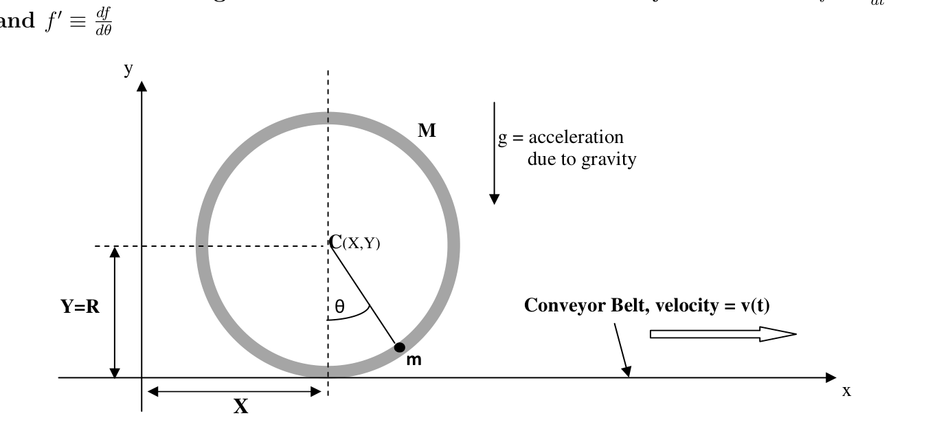
A loaded hoop consists of a ‘load’ or point mass $m$, embedded in a rigid hoop with mass $M$ and radius $R$. The hoop is on a flat horizontal conveyor belt. At time $t$, the load subtends an angle $\theta$ with the vertical while the horizontal and vertical coordinates of the center $C$ of the hoop are $X$ and $Y$ respectively.

In this problem assume that the hoop does not tilt and is always in the same vertical plane. The gravitational acceleration is $g$.

Use the following conventions for the derivatives of any function $f$: $\dot{f}\equiv \frac{df}{dt}\text{and}{f}^{\prime }\equiv \frac{df}{d\theta }$

Part 1. Preliminary Calculations

For Part 1, assume that the hoop is always in contact with the conveyor belt and that $X$ and $\theta$ are independent (i.e. do not assume any constraint such as a non-slip condition etc.).

1.A. Acceleration: Express the horizontal and vertical components, $a_x$ and $a_y$, of the acceleration of the load in the laboratory frame in terms of $R$, $\ddot{X}$, $\theta$, $\dot{\theta }$, and $\ddot{\theta }$.

1.B. Energy: Use the convention that the gravitational potential energy of the loaded hoop is zero when the load is at the bottom. Express the total mechanical energy, $E$, of the loaded hoop in terms of $M$, $m$, $g$, $R$, $\theta$, $\dot{\theta }$, and $\dot{X}$.

Part 2. Oscillation on a Stationary Conveyor Belt

For Part 2 assume that the conveyor belt is at rest. If the loaded hoop is given a small angular displacement from the vertical and released from rest the system will oscillate.

2.A. Period when friction is negligible: Assuming that friction is negligible, determine the period of the small oscillation, $T_A$ of the loaded hoop.

2.B. Period when the hoop does not slip: Assuming that friction is high enough to ensure that there is no sliding, determine the period of small oscillation, $T_B$ of the loaded hoop.

Part 3. Stable Angular Orientations on an Accelerating Conveyor Belt

For Part 3, assume the following:

• The loaded hoop is placed on the conveyor belt at time $t=0$ and initially $\dot{\theta }=\dot{X}=X=0$.
• The velocity at any point of the belt is given by $v=Kt$ where $K$ is a proportionality constant.

If the loaded hoop is placed on the conveyor belt at $t=0$ with carefully chosen initial values of $\theta$, then it will maintain a stable angular orientation provided $K/g$, ${\mu }_s$, ${\mu }_k$, and $m/M$ satisfy appropriate conditions — assume that these conditions are satisfied only in Part 3.

3.A. Determine the stable orientation angle $\theta ={\alpha }_1$ as a function of $m/M$ when $m/M\ge 7$, ${\mu }_k=\sqrt{3}/3$, $K=\sqrt{3}g$ and ${\mu }_s=1.0$.

3.B. Determine the stable orientation angle $\theta ={\alpha }_2$ as a function of $m/M$ when $m/M\ge 7$, ${\mu }_k=\sqrt{3}/3$, $K=\sqrt{3}g$ and ${\mu }_s=2.0$.

Part 4. Oscillation, Rotation, and Sliding on an Accelerating Conveyor Belt

For Part 4, assume the following:

• $M=m$
• The loaded hoop is placed on the conveyor belt at time $t=0$ and initially $\dot{\theta }=\dot{X}=\theta =X=0$.
• The velocity at any point of the belt is given by $v=Kt$ where $K$ is a positive constant.
• Let $\omega \equiv \frac{d}{dt}\theta$.

4.A. When the coefficient of static friction is extremely high (as will be assumed here), two types of motion may ensue:

• Type A: The loaded hoop undergoes angular oscillations forever and never slides.
• Type B: The loaded hoop completes at least one rotation without sliding.

(4.A.1) Type A Motion. For Part 4.A.1, suppose that the loaded hoop is observed to undergo Type A Motion and maximal angular displacement of the load is observed to be ${\theta }_{\text{maximum}}\equiv \beta =30^{\circ }$. Deduce an algebraic expression for $K/g$ in terms of $\beta$ and determine its numerical value.

(4.A.1) Type B Motion. When $K/g$ exceeds a threshold value $\gamma$, the loaded hoop undergoes Type B motion. Determine the numerical value of $\gamma$ to two significant figures.

4.B. Sliding Motion. Now assume that the value of $K/g$ is the same as the value that you were asked to calculate in Part 4.A.1, but this time do not assume that the coefficient of static friction is extremely high. When the coefficient of static friction is less than a threshold value ${\mu }_{s,0}$, the loaded hoop will not undergo Type A motion because it will slide. Determine the numerical value of ${\mu }_{s,0}$ to two significant figures.

Hint: $\frac{d^2}{d{t}^2}\theta =\omega \frac{d\omega }{d\theta }$

Fonte: Testo (PDF) — p.1 Topic: Rotational Dynamics, Oscillations & Waves Metodi: Torque & Angular Momentum Analysis, Free-Body Diagram, Simple Harmonic Motion Analysis, Energy Conservation Method Competenze: Physical Reasoning, Mathematical Modeling Objects: Wheel

Coppi carichi su cintura di trasporto Data limite 31 marzo 2012

Un cerchio carico è costituito da un “carico” o massa puntaria $m$, inserito in un cerchio rigido con massa $M$ e raggio $R$. L’anello è su una cintura di trasporto orizzontale piatta. Al tempo $t$, il carico sottolinea un angolo $\theta$ con la verticale mentre le coordinate orizzontali e verticali del centro $C$ del cerchio sono rispettivamente $X$ e $Y$.

In questo problema supponiamo che l’orlo non si incline e sia sempre nello stesso piano verticale. L’accelerazione gravitazionale è $g$.

Per le derivate di qualsiasi funzione $f$ si utilizzano le seguenti convenzioni: $\dot{f}\equiv \frac{df}{dt}\text{and}{f}^{\prime }\equiv \frac{df}{d\theta }$

Parte 1. Calcoli preliminari

Per quanto riguarda la parte 1, supponiamo che l’orlo sia sempre in contatto con la cintura trasportatrice e che $X$ e $\theta$ siano indipendenti (cioè: non assumono alcuna limitazione come la condizione di non scivolare, ecc.).

**1.A. Accelerazione: ** Esprimere le componenti orizzontali e verticali, $a_x$ e $a_y$, dell’accelerazione del carico nel telaio di laboratorio in termini di $R$, $\ddot{X}$, $\theta$, $\dot{\theta }$ e $\ddot{\theta }$.

1.B. Energia: Utilizzare la convenzione che l’energia potenziale gravitazionale del cerchio carico è zero quando il carico è al fondo. Esprimere l’energia meccanica totale, $E$, del cerchio carico in termini di $M$, $m$, $g$, $R$, $\theta$, $\dot{\theta }$ e $\dot{X}$.

Parte 2. Oscillazione su una cintura di trasporto stazionario

Per la parte 2, supponiamo che la cintura di trasporto sia in riposo. Se il cerchio carico viene spostato in un angolo piccolo dalla verticale e rilasciato dal riposo il sistema oscilla.

**2.A. Periodo in cui l’attrito è trascurabile: ** Supponendo che l’attrito sia trascurabile, determinare il periodo della piccola oscillazione, $T_A$ del cerchio carico.

**2.B. Periodo in cui l’orlo non scivola: ** Supponendo che l’attrito sia sufficientemente elevato per garantire che non vi sia un scivolo, determinare il periodo di piccola oscillazione, $T_B$ dell’orlo carico.

Parte 3. Orientazioni angolari stabili su una cintura di trasporto accelerata

Per quanto riguarda la parte 3, supponiamo quanto segue:

• L’orlo carico viene posizionato sulla cintura trasportatrice al momento $t=0$ e inizialmente $\dot{\theta }=\dot{X}=X=0$.
• La velocità in qualsiasi punto della cintura è data da $v=Kt$, dove $K$ è una costante di proporzionalità.

Se l’orlo carico viene posizionato sulla cintura trasportatrice a $t=0$ con valori iniziali accuratamente scelti di $\theta$, allora manterrà un’orientamento angolare stabile purché $K/g$, ${\mu }_s$, ${\mu }_k$ e $m/M$ soddisfino le condizioni appropriate presumiamo che tali condizioni siano soddisfatte solo nella parte 3.

3.A. Determinare l’angolo di orientamento stabile $\theta ={\alpha }_1$ come funzione di $m/M$ quando $m/M\ge 7$, ${\mu }_k=\sqrt{3}/3$, $K=\sqrt{3}g$ e ${\mu }_s=1.0$.

3.B. Determinare l’angolo di orientamento stabile $\theta ={\alpha }_2$ come funzione di $m/M$ quando $m/M\ge 7$, ${\mu }_k=\sqrt{3}/3$, $K=\sqrt{3}g$ e ${\mu }_s=2.0$.

Parte 4. Oscillazione, rotazione e scivolamento su una cintura di trasporto accelerante

Per quanto riguarda la parte 4, supponiamo quanto segue:

• $M=m$
• L’orlo carico viene posizionato sulla cintura trasportatrice al momento $t=0$ e inizialmente $\dot{\theta }=\dot{X}=\theta =X=0$.
• La velocità in qualsiasi punto della cintura è data da $v=Kt$, dove $K$ è una costante positiva.
• Lasciate $\omega \equiv \frac{d}{dt}\theta$.

4.A. Quando il coefficiente di attrito statico è estremamente elevato (come presumerebbero qui), possono verificarsi due tipi di movimento:

• **Typ A: ** L’ arco carico subisce oscillazioni angolari per sempre e non scivola mai.
• **Typ B: ** L’ arco carico completa almeno una rotazione senza scivolare.

(4.A.1) Typ A Motion. Per la parte 4.A.1, supponiamo che l’orlo carico sia osservato sottoporsi a Motion di tipo A e che il spostamento angolare massimo del carico sia osservato come ${\theta }_{\text{maximum}}\equiv \beta =30^{\circ }$. Riduzione di un’espressione algebrica per $K/g$ in termini di $\beta$ e determinazione del suo valore numerico.

(4.A.1) Tip B Motion. Quando $K/g$ supera un valore soglia $\gamma$, il cerchio carico subisce un movimento di tipo B. Determinare il valore numerico di $\gamma$ a due cifre significative.

4.B. Mozione scorrevole. Ora supponiamo che il valore di $K/g$ sia lo stesso del valore che ti è stato chiesto di calcolare nella parte 4.A.1, ma questa volta non supponiamo che il coefficiente di attrito statico sia estremamente alto. Quando il coefficiente di attrito statico è inferiore a un valore soglia ${\mu }_{s,0}$, l’anello carico non subirà movimento di tipo A perché scivolerà. Determinare il valore numerico di ${\mu }_{s,0}$ a due cifre significative.

*Signore: * $\frac{d^2}{d{t}^2}\theta =\omega \frac{d\omega }{d\theta }$

Fonte: Testo (PDF) — p.1 Topic: Rotational Dynamics, Oscillations & Waves Metodi: Torque & Angular Momentum Analysis, Free-Body Diagram, Simple Harmonic Motion Analysis, Energy Conservation Method Competenze: Physical Reasoning, Mathematical Modeling Objects: Wheel

The Bohr’s molecule — Deadline April 30, 2012

In 1913 Niels Bohr published his famous model of the hydrogen atom explaining for the first time the Rydberg’s formula for the emission spectrum of atomic hydrogen. According to the Bohr’s model, the electron in the hydrogen atom revolves around the positively charged nucleus along one of the allowed ‘stationary’ orbits satisfying the condition: L = n\frac{h}{2\pi}, \tag{1} where $L$ is the electron’s angular momentum, $n=1,2,\dots$ is a positive integer number, and $h=6.626\times 10^{-34}\text{J⋅s}$ is the Planck’s constant. For the sake of simplicity we will use also the ‘reduced’ Planck’s constant $\hslash =1.055\times 10^{-34}\text{J⋅s}$. Thus, the quantization condition (1) could be rewritten in the form: L = n\hbar. \tag{2}

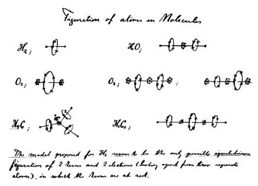Figure 1: Stationary electronic orbits for different molecules as suggested by Niels Bohr in 1913.

Inspired by the agreement between the theoretical predictions of his model and the experimental data for the hydrogen atom, Niels Bohr has made an attempt to apply the concept of stationary orbit to more complicated systems like many-electron atoms and molecules. Figure 1 represents an original sketch by Niels Bohr of possible stationary electron orbits in a number of molecules. For the suggested molecular models, however, Bohr did not observe precise agreement with the experimental data concerning the distances between atomic protons and the molecular bonding energies.

The interest in the Bohr’s molecular model, however, has revived after a number of recent publications showing that there is a larger variety of stationary orbits in the hydrogen molecule than originally suggested by Niels Bohr. It was demonstrated that by using different sets of orbits the Bohr’s model provides a computationally non-demanding method for an approximate calculation of the molecular properties. In this problem you are going to investigate some physical characteristics of the hydrogen molecule as predicted by the original model of Bohr.

Description of the Bohr’s model for H₂ molecule

Shown in Figure 2 is a detailed sketch of the model of the hydrogen molecule proposed by Niels Bohr. The two protons ($p^{+}$) are separated by a distance $R$. The two electrons ($e^{-}$) revolve with the same angular velocity around the same circular orbit, which is perpendicular to and bisects the line connecting the two protons. The electron-proton distances are denoted by $r$, and the radius of the circular orbit by $\rho$.

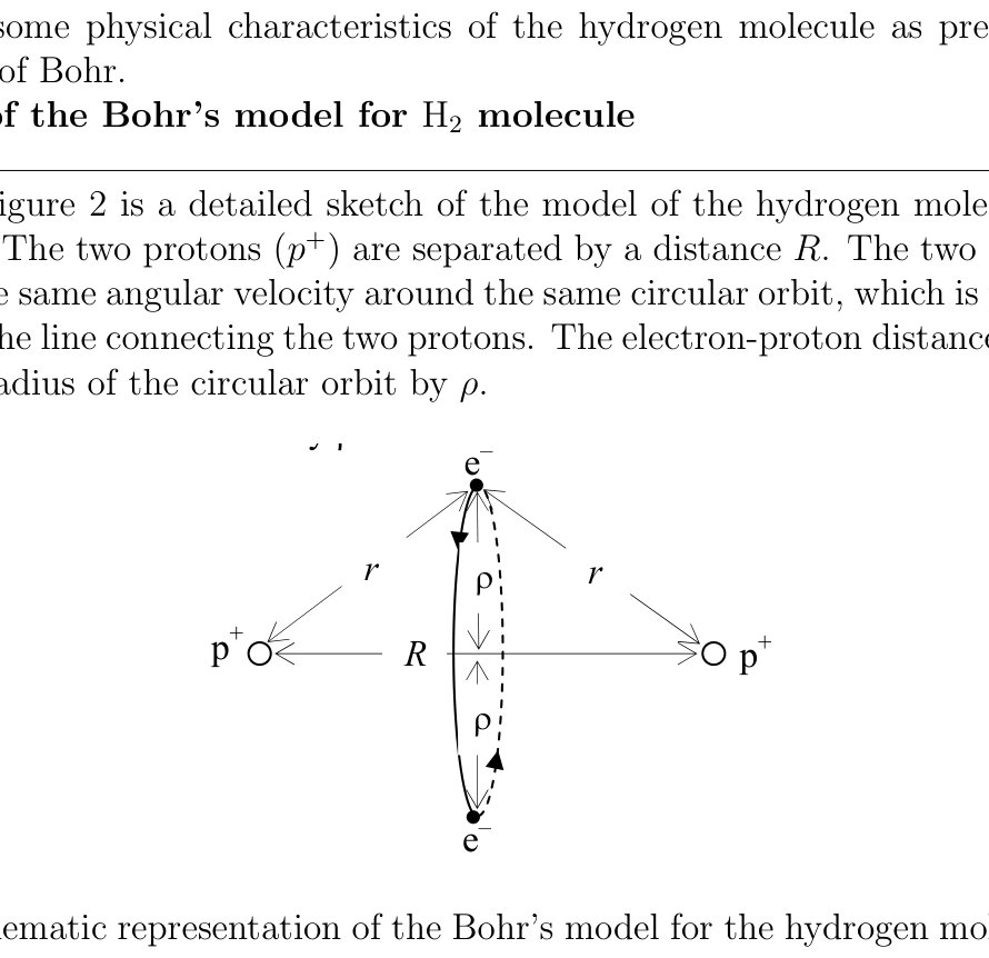Figure 2: A schematic representation of the Bohr’s model for the hydrogen molecule. Shown are all the relevant distances.

It is assumed that:

• The electrons move according to the Newton’s laws of dynamics.
• The quantization condition (2) is satisfied by each of the electrons.
• The electrons lie on a same diameter of the circular orbit.

List of available physical constants

• Elementary electric charge: $e=1.602\times 10^{-19}\text{C}$
• Coulomb’s constant: $k=\frac{1}{4\pi {ϵ}_0}=8.988\times 10^9{\text{N⋅m}}^2/{\text{C}}^2$
• Electric permittivity of vacuum: ${ϵ}_0=8.854\times 10^{-12}\text{F/m}$
• Reduced Planck’s constant: $\hslash =\frac{h}{2\pi }=1.055\times 10^{-34}\text{J⋅s}$
• Mass of the electron: $m_e=9.109\times 10^{-31}\text{kg}$
• Mass of the proton: $m_p=1.673\times 10^{-27}\text{kg}$
• Speed of light: $c=2.998\times 10^8\text{m/s}$

Part 1. H₂ molecule in equilibrium

In this task we assume that the two protons are at rest in their equilibrium positions.

1.A. Calculate the ratios $r/R$ and $\rho /R$ for a molecule with protons in equilibrium.

1.B. Derive an expression for the electric potential energy $E_p$ of the molecule in terms of the internuclear distance $R$ and the available physical constants.

1.C. Calculate the ratio $E_k/E_p$ of the total kinetic energy of electrons to the potential energy of the molecule provided that the protons are in equilibrium positions.

1.D. Derive an expression for the minimum distance $R_0$ between protons in equilibrium in terms of the provided constants. Calculate the numerical value of $R_0$.

The bonding energy $E_b$ of a molecule is defined as the minimum energy required to dissociate the molecule into electrically neutral atoms separated by an infinite distance from each other.

1.E. Calculate the bonding energy $E_b$ of the hydrogen molecule as predicted by the Bohr’s model. You can use the ionization energy of the hydrogen atom, $E_I=13.606\text{eV}$.

Part 2. Vibrating H₂ molecule

In practice atomic nuclei in a molecule are not at rest but vibrate around their equilibrium positions. These vibrations persist even at temperatures close to $0\text{K}$ due to the quantum nature of atomic motion. Therefore, as the temperature tends to $0\text{K}$, the energy and the amplitude of atomic vibrations tend to specific minimum values.

Since the protons are much heavier than the electrons, the velocities of the electrons in a molecule are several orders of magnitude higher than the nuclear velocities. For that reason, it is assumed in molecular physics that in each moment of time the electrons move along stationary orbits corresponding to the instantaneous positions of the protons as if the latter were at rest. According to this approximation the effective potential energy $E$ of the hydrogen molecule (does not include the kinetic energy of the protons) is a function of the instantaneous distance $R$ between protons. The effective potential energy of the molecule when the atoms are at an infinite distance is taken to be zero. It is not possible to derive an exact expression for the function $E(R)$ even in the frame of the Bohr’s model. Instead, this function can be approximated by several expressions, whose applicability is justified on an experimental basis. In this task we will adopt the so called Morse function: E(R) = D\left(e^{2\alpha(1-R/R_0)} - 2e^{\alpha(1-R/R_0)}\right) \tag{3} where $D$ and $\alpha$ are positive constants.

Remark: If you did not calculate $R_0$ and $E_b$ in points (1D) and (1E), use in this task the following values instead: $R_0=0.6\text{A˚}$ and $E_b=3.0\text{eV}$.

2.A. Sketch qualitatively a graph of the Morse function. Indicate on the graph the equilibrium distance $R_0$ between protons and the bonding energy $E_b$ of the molecule.

2.B. Write down a relation between the constant $D$ and the bonding energy $E_b$.

We will consider the vibrations of the protons in the H₂ molecule in a reference frame where the molecular center-of-mass is at rest. Assume that the displacements of the protons from their equilibrium positions are much smaller than the distance $R_0$.

2.C. Derive an expression for the linear frequency ${\nu }_{\text{vib}}$ of vibration of the hydrogen molecule in terms of $\alpha$, $R_0$, $E_b$, and the proton mass $m_p$.

One of the experimental techniques used to measure the frequency of molecular oscillations is known as Raman spectroscopy. According to quantum mechanics, each system vibrating with a frequency ${\nu }_{\text{vib}}$ can exchange energy only in discrete quanta $h{\nu }_{\text{vib}}$. Raman scattering is a process in which an incident photon of a specific wavelength ${\lambda }_i$ interacts with a molecule and transfers to it one quantum of vibrational energy. As a result, the photon scatters away with a wavelength ${\lambda }_s$ larger than the initial wavelength ${\lambda }_i$. In the Raman process the energy transformed into translational and rotational motion of the molecule is several orders of magnitude smaller than the energy transferred to vibration.

In a particular experiment an ampoule containing molecular hydrogen is illuminated with a monochromatic light of wavelength ${\lambda }_i=514\text{nm}$. It has been established that there is a weak scattered light from the ampoule with a wavelength ${\lambda }_s=664\text{nm}$.

2.D. Calculate numerically ${\nu }_{\text{vib}}$ and determine the value of the constant $\alpha$ in the Morse function.

2.E. Make an order of magnitude estimate of the minimum possible amplitude $A_{\min }$ of the vibrations of protons in the hydrogen molecule.

Fonte: Testo (PDF) — p.1 Topic: Modern-Quantum Physics, Oscillations & Waves Metodi: Bohr Model & Quantization, Coulomb’s Law, Photon Energy Relation, Simple Harmonic Motion Analysis Competenze: Physical Reasoning, Mathematical Modeling, Estimation & Approximation Objects: Atom, Electron, Nucleus, Photon

The Bohr’s molecule — Deadline April 30, 2012

Nel 1913 Niels Bohr pubblicò il suo famoso modello dell’atomo di idrogeno spiegando per la prima volta la formula di Rydberg per lo spettro di emissioni dell’idrogeno atomico. Secondo il modello di Bohr, l’elettrone nell’atomo di idrogeno ruota intorno al nucleo carico positivamente lungo una delle orbite ‘stazionarie’ consentite soddisfacendo la condizione: L = n\frac{h}{2\pi}, \tag{1} dove $L$ è il momento angolare dell’elettrone, $n=1,2,\dots$ è un numero intero positivo e $h=6.626\times 10^{-34}\text{J⋅s}$ è la costante di Planck. Per semplificazione, utilizzeremo anche la costante di Planck $\hslash =1.055\times 10^{-34}\text{J⋅s}$ “ridotta”. La condizione di quantizzazione (1) potrebbe quindi essere riscritta sotto la forma: L = n\hbar. \tag{2}

**Figura 1: ** Orbit elettroniche stazionarie per diverse molecole come suggerito da Niels Bohr nel 1913.

Ispirato all’accordo tra le previsioni teoriche del suo modello e i dati sperimentali per l’atomo di idrogeno, Niels Bohr ha tentato di applicare il concetto di orbita stazionaria a sistemi più complessi come atomi e molecole a molti elettroni. La figura 1 rappresenta uno sketch originale di Niels Bohr di possibili orbite di elettroni stazionari in un certo numero di molecole. Per i modelli molecolari suggeriti, tuttavia, Bohr non osservò un accurato accordo con i dati sperimentali riguardanti le distanze tra i protoni atomici e le energie di legame molecolare.

L’interesse per il modello molecolare di Bohr, tuttavia, è risvegliato dopo una serie di recenti pubblicazioni che mostrano che c’è una maggiore varietà di orbite stazionarie nella molecola di idrogeno di quanto originariamente suggerito da Niels Bohr. È stato dimostrato che utilizzando diversi set di orbite il modello di Bohr fornisce un metodo non richiesto dal punto di vista computazionale per un calcolo approssimativo delle proprietà molecolari. In questo problema si esamineranno alcune caratteristiche fisiche della molecola di idrogeno come previsto dal modello originale di Bohr.

Descrizione del modello di Bohr per la molecola H2

Nella figura 2 è mostrato uno schizzo dettagliato del modello della molecola di idrogeno proposto da Niels Bohr. I due protoni ($p^{+}$) sono separati da una distanza $R$. I due elettroni ($e^{-}$) ruotano con la stessa velocità angolare intorno alla stessa orbita circolare, che è perpendicolare e divide la linea che collega i due protoni. Le distanze tra elettroni e protoni sono indicate da $r$ e il raggio dell’orbita circolare da $\rho$.

**Figura 2: ** Una rappresentazione schematica del modello di Bohr per la molecola di idrogeno. Sono mostrate tutte le distanze pertinenti.

Si presume che:

Gli elettroni si muovono secondo le leggi di Newton.

• La condizione di quantizzazione (2) è soddisfatta da ciascun elettrone.
• Gli elettroni si trovano sullo stesso diametro dell’orbita circolare.

Lista delle costanti fisiche disponibili

• carica elettrica elementare: $e=1.602\times 10^{-19}\text{C}$
• Costante di Coulomb: $k=\frac{1}{4\pi {ϵ}_0}=8.988\times 10^9{\text{N⋅m}}^2/{\text{C}}^2$
• Permissibilità elettrica del vuoto: ${ϵ}_0=8.854\times 10^{-12}\text{F/m}$
• Costante di Planck ridotta: $\hslash =\frac{h}{2\pi }=1.055\times 10^{-34}\text{J⋅s}$
• Massa dell’elettrone: $m_e=9.109\times 10^{-31}\text{kg}$
• Massa del protone: $m_p=1.673\times 10^{-27}\text{kg}$
• Velocità della luce: $c=2.998\times 10^8\text{m/s}$

Parte 1. Molcole di H2 in equilibrio

In questo compito supponiamo che i due protoni siano a riposo nelle loro posizioni di equilibrio.

1.A. Calcolare i rapporti $r/R$ e $\rho /R$ per una molecola con protoni in equilibrio.

1.B. Derivare un’espressione per l’energia elettrica potenziale $E_p$ della molecola in termini di distanza internucleare $R$ e delle costanti fisiche disponibili.

1.C. Calcolare il rapporto $E_k/E_p$ tra l’energia cinetica totale degli elettroni e l’energia potenziale della molecola a condizione che i protoni siano in posizione di equilibrio.

1.D. Derivare un’espressione per la distanza minima $R_0$ tra i protoni in equilibrio in termini di costanti fornite. Calcolare il valore numerico di $R_0$.

L’energia di legame $E_b$ di una molecola è definita come l’energia minima necessaria per dissociare la molecola in atomi elettricamente neutrali separati da una distanza infinita tra loro.

1.E. Calcolare l’energia di legame $E_b$ della molecola di idrogeno come previsto dal modello di Bohr. Si può usare l’energia di ionizzazione dell’atomo di idrogeno, $E_I=13.606\text{eV}$.

Parte 2. Molcole di H2 in vibrazione

In pratica i nuclei atomici di una molecola non sono a riposo ma vibranti intorno alle loro posizioni di equilibrio. Queste vibrazioni persistono anche a temperature vicine a $0\text{K}$ a causa della natura quantistica del movimento atomico. Pertanto, poiché la temperatura tende a $0\text{K}$, l’energia e l’ampiezza delle vibrazioni atomiche tendono a valori minimi specifici.

Poiché i protoni sono molto più pesanti degli elettroni, le velocità degli elettroni in una molecola sono di diversi ordini di grandezza superiori alle velocità nucleari. Per questo motivo, nella fisica molecolare si assume che in ogni momento del tempo gli elettroni si muovono lungo orbite stazionarie corrispondenti alle posizioni istantanee dei protoni come se questi ultimi fossero in riposo. Secondo questa approssimazione l’energia potenziale effettiva $E$ della molecola di idrogeno (non include l’energia cinetica dei protoni) è una funzione della distanza istantanea $R$ tra i protoni. L’energia potenziale efficace della molecola quando gli atomi sono a una distanza infinita è considerata zero. Non è possibile derivare un’espressione esatta per la funzione $E(R)$ anche nel quadro del modello di Bohr. Invece, questa funzione può essere approssimata da diverse espressioni, la cui applicabilità è giustificata su base sperimentale. In questo compito adotteremo la cosiddetta funzione di Morse: E(R) = D\left(e^{2\alpha(1-R/R_0)} - 2e^{\alpha(1-R/R_0)}\right) \tag{3} dove $D$ e $\alpha$ sono costanti positive.

*Ricerca: * Se non si calcola $R_0$ e $E_b$ nei punti (1D) e (1E), utilizzare in questo compito i seguenti valori: $R_0=0.6\text{A˚}$ e $E_b=3.0\text{eV}$.

2.A. Segna qualitativamente un grafico della funzione Morse. Indicare sul grafico la distanza di equilibrio $R_0$ tra i protoni e l’energia di legame $E_b$ della molecola.

2.B. Scrivi una relazione tra la costante $D$ e l’energia di legame $E_b$.

Considereremo le vibrazioni dei protoni nella molecola H2 in un quadro di riferimento in cui il centro molecolare di massa è a riposo. Supponiamo che i spostamenti dei protoni dalle loro posizioni di equilibrio siano molto più piccoli della distanza $R_0$.

2.C. Derivare un’espressione per la frequenza lineare ${\nu }_{\text{vib}}$ di vibrazione della molecola di idrogeno in termini di $\alpha$, $R_0$, $E_b$ e della massa dei protoni $m_p$.

Una delle tecniche sperimentali utilizzate per misurare la frequenza delle oscillazioni molecolari è conosciuta come spettroscopia Raman. Secondo la meccanica quantistica, ogni sistema che vibra con una frequenza ${\nu }_{\text{vib}}$ può scambiare energia solo in quanti discreti $h{\nu }_{\text{vib}}$. La dispersione di Raman è un processo in cui un fotone incidente di una lunghezza d’onda specifica ${\lambda }_i$ interagisce con una molecola e trasferisce a essa un quantum di energia vibrazionale. Di conseguenza, il fotone si disperde con una lunghezza d’onda ${\lambda }_s$ maggiore della lunghezza d’onda iniziale ${\lambda }_i$. Nel processo di Raman l’energia trasformata in movimento traslazionale e rotazionale della molecola è di diversi ordini di magnitudo inferiore all’energia trasferita alla vibrazione.

In un esperimento particolare, un’ampolla contenente idrogeno molecolare viene illuminata con una luce monocromatica di lunghezza d’onda ${\lambda }_i=514\text{nm}$. È stato stabilito che l’ampolla produce una luce scatenata debole con una lunghezza d’onda ${\lambda }_s=664\text{nm}$.

2.D. Calcolare numericamente ${\nu }_{\text{vib}}$ e determinare il valore della costante $\alpha$ nella funzione Morse.

2.E. Fare una stima di ordine di magnitudine dell’ampiezza minima possibile $A_{\min }$ delle vibrazioni dei protoni nella molecola di idrogeno.

Fonte: Testo (PDF) — p.1 Topic: Modern-Quantum Physics, Oscillations & Waves Metodi: Bohr Model & Quantization, Coulomb’s Law, Photon Energy Relation, Simple Harmonic Motion Analysis Competenze: Physical Reasoning, Mathematical Modeling, Estimation & Approximation Objects: Atom, Electron, Nucleus, Photon

Heat capacity of moist porous solid — Deadline April 30, 2012

When fabricated or in use, solid porous bodies may be exposed to moisture penetrating their pores in a form of difficult-to-remove water. In this problem, you are asked to investigate the moisture content influence on thermal properties of porous solids.

The porous solid considered in the problem contains only closed pores with a little amount of water in them (Fig. 1). A volume of liquid water is negligible compared to that of the pore. The water is in equilibrium with the vapour phase. For simplicity the pores are taken to be void of any other gases. The pore heat expansion also can be neglected.

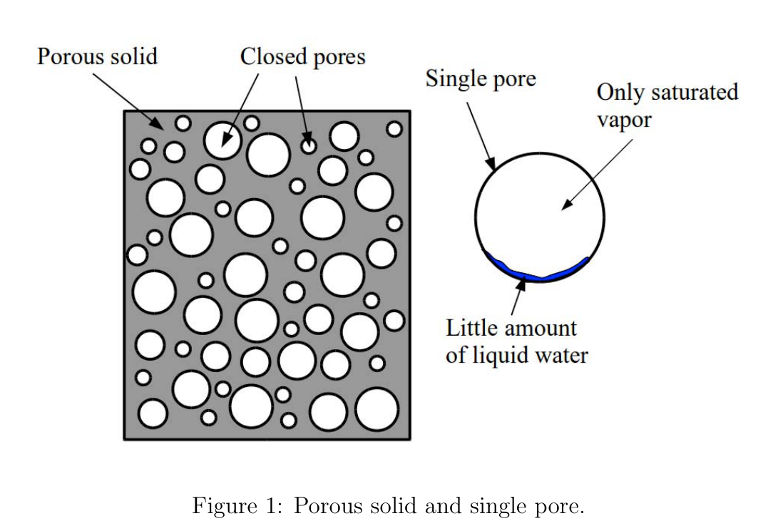Figure 1: Porous solid and single pore.

Part 1. Pore contents

To begin with, consider processes involving a liquid and vapour in a single pore. Let an amount of liquid water with mass $m_{W0}$ be in the pore of the volume $V$. The saturated vapour pressure is $p_0$, temperature is $T_0$. The molar mass of water is $M$, specific heat capacity is $c_W$, specific heat of evaporation is $L$. The vapour molar heat capacity at constant volume is $3R$. Assume that the specific heat capacity, specific heat of evaporation, and vapour molar heat capacity do not depend on temperature and pressure.

1.A. Find the mass of vapour $m_{S0}$ in the pore.

On heating a fraction of water evaporates and the vapour content in the pore increases. The saturated vapour pressure depends on temperature as follows: p = p_0\, e^{\frac{ML}{R}\left(\frac{1}{T_0} - \frac{1}{T}\right)}, \tag{1} where $p_0$ is the pressure at temperature $T_0$.

The saturated vapour pressure variation near a curved surface of water can be neglected.

1.B. How do the masses of vapour and liquid water depend on temperature ($m_W(T)$ and $m_S(T)$)?

Let the vapour mass be equal to $m_S$ at a certain temperature $T$. The temperature of pore content increases from $T$ to $T+\Delta T$.

1.C. Considering the temperature change to be small ($\Delta T/T\ll 1$), write down the expression for the vapour mass change ($\Delta m_S(T)$).

Hint. Use the following approximations valid for $x\ll 1$: e^x \approx 1 + x \qquad \text{and} \qquad (1+x)^\alpha \approx 1 + \alpha x. \tag{2}

1.D. How does the heat capacity $C_P(T)$ of the pore contents depend on temperature? Assume that the water does not evaporate completely.

At temperature $T_0=3.0\times 10^2\text{K}$, the saturated vapour pressure is $P_0=3.5\text{kPa}$ and liquid water occupies $\delta =0.3\%$ of the pore volume. The water molar mass is $M=18\times 10^{-3}\text{kg/mole}$, the density is ${\rho }_w=9.5\times 10^2{\text{kg/m}}^3$, the specific heat capacity is $c_w=4.2\times 10^3\text{J/K⋅mole}$ and the specific heat of evaporation is $L=2.3\times 10^6\text{J/kg}$. Universal gas constant is $R=8.3\text{J/K⋅mole}$. Assume that the density does not depend on temperature and pressure.

1.E. At what temperature $T_1$ will water completely evaporate? You can calculate the value of the temperature numerically.

1.F. Estimate the values of all terms in the expression for heat capacity of pore content $C_P(T)$. Write down the expression for $C_P(T)$ retaining only the two most significant summands. What is the physical meaning of these terms?

Let’s define the specific heat capacity of the pore contents as a ratio of heat capacity of the pore contents to the mass of the pore contents: c_p = \frac{C_p}{m_W + m_S} \tag{3}

1.G. Calculate the values of the specific heat capacity for the pore contents at $T=T_0$, $T\to T_1$, and $T>T_1$.

Part 2. Porous solid

In this part, you should solve the problem by taking into account properties of the porous body.

Let the porosity (a ratio of the volume of pores to the total body volume) be $\xi =2/3$. The density of a body skeletal portion is ${\rho }_S=6.0\times 10^2{\text{kg/m}}^3$ and its specific heat capacity is $C_S=4.0\times 10^2\text{J/kg⋅K}$. Initial conditions for the pore contents are the same as in part 1: $\delta =0.30\%$, $T_0=3.0\times 10^2\text{K}$, and $p_0=3.5\text{kPa}$.

2.A. Write down the expression for the specific heat capacity $c(T)$ of the moist porous solid.

2.B. Find numerical values of the specific heat capacity of porous solid at $T=T_0$, $T\to T_1$ and $T>T_1$.

2.C. Plot the specific heat capacity versus temperature for $T\in (T_0;T>T_1)$.

Fonte: Testo (PDF) — p.1 Topic: Thermodynamics, Kinetic Theory Metodi: First Law of Thermodynamics, Ideal Gas Law, Approximation & Series Expansion, Physical Modeling Competenze: Physical Reasoning, Estimation & Approximation Objects: Gas

Capacità termico di solido poroso umido Termine 30 aprile 2012

Quando sono fabbricati o utilizzati, i corpi solidi porosi possono essere esposti all’umidità che penetra nei loro pori sotto forma di acqua difficile da rimuovere. In questo problema, si chiede di esaminare l’influenza del contenuto di umidità sulle proprietà termiche dei solidi porosi.

Il solido poroso considerato nel problema contiene solo pori chiusi con una piccola quantità di acqua (Fig. 1). Un volume di acqua liquida è insignificante rispetto a quello del poro. L’acqua è in equilibrio con la fase di vapore. Per semplicità, i pori sono considerati privi di qualsiasi altro gas. Anche l’espansione del calore dei pori può essere trascurata.

**Figura 1: ** solido poroso e poroso singolo.

Parte 1. Contenuto delle porche

Per cominciare, consideriamo i processi che coinvolgono un liquido e vapore in un solo poro. La quantità di acqua liquida con massa $m_{W0}$ deve essere nel porone del volume $V$. La pressione di vapore saturazione è $p_0$, la temperatura è $T_0$. La massa molare dell’acqua è $M$, la capacità termico specifica è $c_W$, il calore specifico di evaporazione è $L$. La capacità di calore molare del vapore a volume costante è $3R$. Supponiamo che la capacità di calore specifica, la capacità di calore specifica di evaporazione e la capacità di calore molare del vapore non dipendano dalla temperatura e dalla pressione.

1.A. Trova la massa del vapore $m_{S0}$ nel poro.

Il riscaldamento fa evaporare una frazione dell’acqua e aumenta il contenuto di vapore nei pori. La pressione di vapore saturazione dipende dalla temperatura come segue: p = p_0\, e^{\frac{ML}{R}\left(\frac{1}{T_0} - \frac{1}{T}\right)}, \tag{1} dove $p_0$ è la pressione a temperatura $T_0$.

La variazione della pressione del vapore saturo vicino a una superficie curva dell’acqua può essere trascurata.

1.B. How do the masses of vapour and liquid water depend on temperature ($m_W(T)$ and $m_S(T)$)?

La massa del vapore deve essere pari a $m_S$ a una certa temperatura $T$. La temperatura del contenuto dei pori aumenta da $T$ a $T+\Delta T$.

1.C. Considerando che il cambiamento di temperatura è piccolo ($\Delta T/T\ll 1$), annotare l’espressione per il cambiamento di massa del vapore ($\Delta m_S(T)$).

Signore. Utilizzare le seguenti approssimazioni valide per $x\ll 1$: e^x \approx 1 + x \qquad \text{and} \qquad (1+x)^\alpha \approx 1 + \alpha x. \tag{2}

1.D. How does the heat capacity $C_P(T)$ of the pore contents depend on temperature? Supponiamo che l’acqua non evapori completamente.

A temperatura $T_0=3.0\times 10^2\text{K}$, la pressione di vapore saturazione è $P_0=3.5\text{kPa}$ e l’acqua liquida occupa $\delta =0.3\%$ del volume dei pori. La massa molare dell’acqua è $M=18\times 10^{-3}\text{kg/mole}$, la densità è ${\rho }_w=9.5\times 10^2{\text{kg/m}}^3$, la capacità termico specifica è $c_w=4.2\times 10^3\text{J/K⋅mole}$ e il calore specifico di evaporazione è $L=2.3\times 10^6\text{J/kg}$. Costante universale del gas è $R=8.3\text{J/K⋅mole}$. Supponiamo che la densità non dipenda dalla temperatura e dalla pressione.

1.E. At what temperature $T_1$ will water completely evaporate? Puoi calcolare il valore della temperatura numericamente.

1.F. Estimare i valori di tutti i termini nell’espressione per la capacità termico del contenuto di pori $C_P(T)$. Scrivere l’espressione per $C_P(T)$ che conserva solo le due sommand più significative. Qual è il significato fisico di questi termini?

Definitiamo la capacità termico specifica del contenuto dei pori come rapporto tra la capacità termico del contenuto dei pori e la massa del contenuto dei pori: c_p = \frac{C_p}{m_W + m_S} \tag{3}

1.G. Calcolare i valori della capacità termica specifica dei porosi a $T=T_0$, $T\to T_1$ e $T>T_1$.

Parte 2. Fossido poroso

In questa parte, si dovrebbe risolvere il problema tenendo conto delle proprietà del corpo poroso.

La porosità (il rapporto tra il volume dei pori e il volume totale del corpo) deve essere $\xi =2/3$. La densità di una parte dello scheletro corporeo è ${\rho }_S=6.0\times 10^2{\text{kg/m}}^3$ e la sua capacità termico specifica è $C_S=4.0\times 10^2\text{J/kg⋅K}$. Le condizioni iniziali per il contenuto dei pori sono le stesse di quelle della parte 1: $\delta =0.30\%$, $T_0=3.0\times 10^2\text{K}$ e $p_0=3.5\text{kPa}$.

2.A. Scrivere l’espressione per la capacità termico specifica $c(T)$ del solido poroso umido.

2.B. Trovare valori numerici della capacità termica specifica di solido poroso a $T=T_0$, $T\to T_1$ e $T>T_1$.

2.C. Tracciare la capacità termico specifica rispetto alla temperatura per $T\in (T_0;T>T_1)$.

Fonte: Testo (PDF) — p.1 Topic: Thermodynamics, Kinetic Theory Metodi: First Law of Thermodynamics, Ideal Gas Law, Approximation & Series Expansion, Physical Modeling Competenze: Physical Reasoning, Estimation & Approximation Objects: Gas

The Rainbow — Deadline May 31, 2012

The rainbow is a spectacular show of the dispersion phenomenon. There are many beautiful tales about the rainbow, but here we will look at the rainbow from a point of view of Physics. Just after rain, there are still a lot of tiny water droplets in the air. If the sun appears from behind the clouds at this time, then the rainbow can be formed from the sunlight refracted and reflected by these tiny water droplets. Water droplets in the air may have different shapes. Only spherical water droplets make contribution to the formation of the rainbow. When falling down through the air, the shape of a water droplet depends on its size. During that process, the surface tension of the water tends to minimize the surface of the droplet and make the droplet spherical, but at the same time, the weight of the droplet and the air resistant force make the water droplet deform from the spherical shape. The surface tension predominates in smaller water droplets, so smaller water droplets are spherical. For larger water droplets, the weight of the droplet and the air resistant force are stronger than the surface tension, therefore larger water droplets are non-spherical.

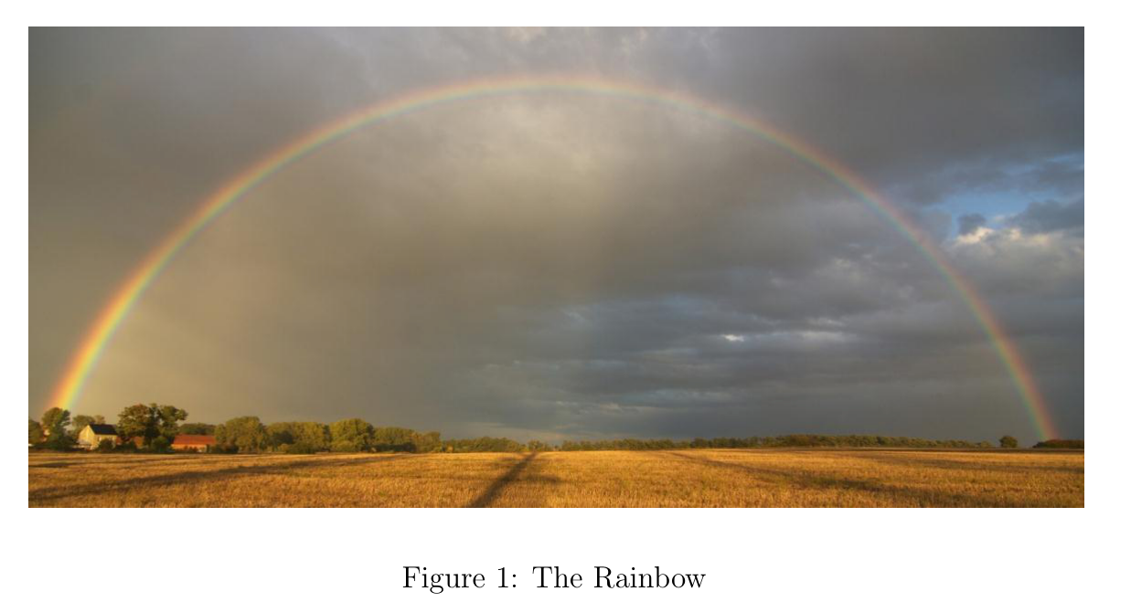Figure 1: The Rainbow

Part 1. The maximal diameter of a spherical water droplet

Consider now a spherical water droplet that falls down through the air with a constant speed. The air resistant force at each point on the surface of the water droplet is tangent to the surface. To simplify the analysis, we assume that the air resistant force is homogeneously distributed over the whole surface of the spherical water droplet (Fig. 2).

1.A. Calculate the air resistant force per unit water droplet surface $f$. Express your result in terms of the density of the water $\rho$, the gravitational acceleration $g$ and the diameter of the water droplet $D$.

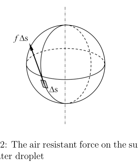Figure 2: The air resistant force on the surface of a water droplet.

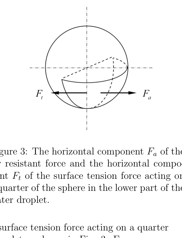Figure 3: The horizontal component $F_a$ of the air resistant force and the horizontal component $F_t$ of the surface tension force acting on a quarter of the sphere in the lower part of the water droplet.

1.B. Calculate the horizontal component $F_a$ of the air resistant force acting on a quarter of the sphere in the lower part of the water droplet as shown in Fig. 3. Express your result in terms of $\rho$, $g$ and $D$.

1.C. Calculate the horizontal component $F_t$ of the surface tension force acting on a quarter of the sphere in the lower part of the water droplet as shown in Fig. 3. Express your result in terms of the surface tension coefficient of water $\sigma$ and $D$.

1.D. When $F_t\gg F_a$ the water droplets are spherical. By using $F_t\ge 100F_a$ as the condition for spherical water droplets, find the maximal diameter of a spherical water droplet $D_M$. ($\sigma =7.5\times 10^{-2}\text{N/m}$, $\rho =1.0\times 10^3{\text{kg/m}}^3$, $g=9.8{\text{m/s}}^2$)

Part 2. Refraction and reflection of light rays in a spherical water droplet

2.A. Consider a light ray that is refracted into the water droplet, then reflected back once in the water droplet, and finally refracted into air, as shown in Fig. 4. $\alpha$ is the central angle of the incident point. Find the angle $\theta$ between the reflected ray and the reverse direction of the incident ray. Express your result in terms of $\alpha$ and the refraction index of water $n$.

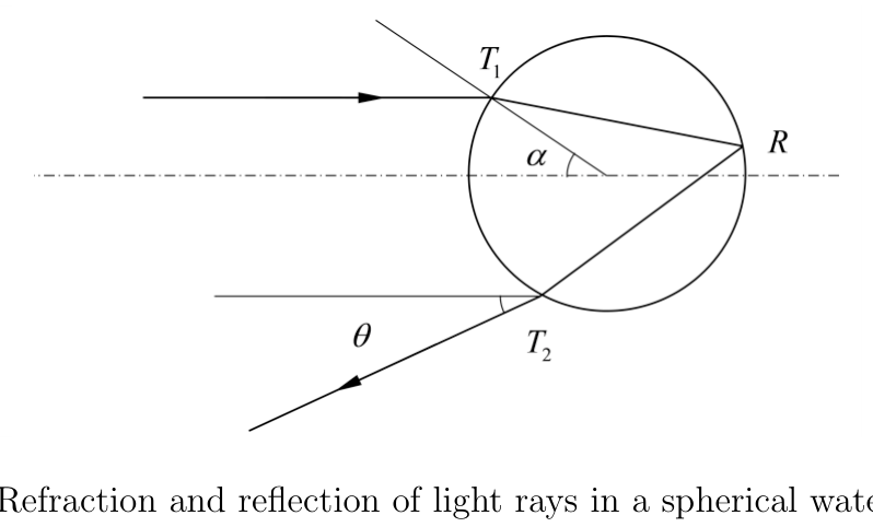Figure 4: Refraction and reflection of light rays in a spherical water droplet.

2.B. Suppose that the incident light is a parallel light with an optical intensity (optical power per unit section) equal to $I_0$. Find the angular optical power distribution of the reflected light $J(\theta )={\lim }_{\begin{array}{c}\Delta \theta \to 0\\ \Delta \phi \to 0\end{array}}\frac{\Delta P}{\Delta \theta \Delta \phi },$ where $\Delta P$ is the optical power within a small angular range $\Delta \phi \Delta \theta$ around a given direction (Fig. 5). Express your result in terms of $\alpha$, $n$, $I_0$, the diameter of the water droplet $D$, the transmittance from air to water $T_1$, the transmittance from water to air $T_2$, the reflectivity in the water droplet $R$.

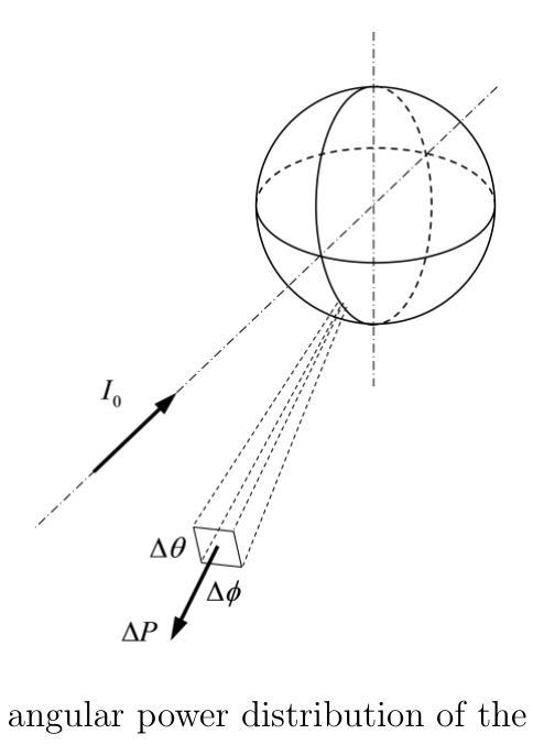Figure 5: The angular power distribution of the reflected light.

2.C. For monochromatic lights with the wavelength $\lambda =550\text{nm}$, calculate the angle ${\theta }_M$ at which the maximum for $J(\theta )$ occurs, and the maximum value $J({\theta }_M)$ of $J(\theta )$. The water’s refraction index at $\lambda =550\text{nm}$ is $n_g=1.3342$.

2.D. Suppose that the incident light is white light that contains all optical waves with the wavelength within the range $390\text{nm}-780\text{nm}$, with equal intensities. Sketch the intensity of the spectrum of the sunlight as a function of wavelength, reflected along the direction $\theta ={\theta }_M$, and indicate special values on the curve.

Part 3. Basic characteristics of the rainbow

3.A. The electromagnetic waves with the wavelength between $390\text{nm}-780\text{nm}$ are visible lights. The water’s refraction index is $n_v=1.3439$ at $\lambda =390\text{nm}$, and $n_r=1.3316$ at $\lambda =780\text{nm}$. The angular diameter of the sun is $\delta =0.5^{\circ }$. Calculate the angular radius ${\theta }_0$ and the angular width $\Delta \theta$ of the rainbow. Assuming the sun is right behind the observer.

3.B. The reflected sunlight is also diffracted by water droplets. The diffraction pattern resulting from a water droplet is the same as the diffraction pattern resulting from a circular aperture with the same diameter as the droplet. If the angular radius of the diffraction pattern resulting from a water droplet is larger than the angular width of the rainbow, then the sunlight reflected from this water droplet does not contribute to the formation of the rainbow. Calculate the diameter $d_m$ of the smallest water droplet that may contribute to rainbow formation.

3.C. If the altitude of the bottom of clouds was $800\text{m}$ during the rain, calculate the maximum time $T_M$ after the rain stopped, the water droplets that can contribute to rainbow formation may still be found at altitudes higher than $200\text{m}$. (The viscosity of the air is $\eta =1.8\times 10^{-5}\text{Pa⋅s}$).

3.D. One afternoon, the rainbow appeared in a certain location. If the day length was $14$ hours for that day, calculate the maximum time $T_r$ (in hours) in which the rainbow could be seen in that afternoon.

Useful formula: $\frac{d}{dx}\arcsin (x)=\frac{1}{\sqrt{1-x^2}}$

Fonte: Testo (PDF) — p.1 Topic: Geometric Optics, Wave Optics Metodi: Snell’s Law, Ray Tracing, Interference & Diffraction Analysis, Calculus-Integration Competenze: Physical Reasoning, Mathematical Modeling Objects: Droplet

L’arcobaleno Data limite 31 maggio 2012

L’arcobaleno è uno spettacolare spettacolo del fenomeno della dispersione. Ci sono molte belle storie sull’arcobaleno, ma qui vedremo l’arcobaleno dal punto di vista della fisica. Dopo la pioggia, ci sono ancora un sacco di piccole gocce d’acqua nell’aria. Se il sole appare da dietro le nuvole in questo momento, allora l’arcobaleno può essere formato dalla luce solare refrattata e riflessa da queste piccole gocce d’acqua. Le goccioline d’acqua nell’aria possono avere forme diverse. Solo gocce di acqua sferiche contribuiscono alla formazione dell’arcobaleno. Quando cade attraverso l’aria, la forma di una goccia d’acqua dipende dalla sua dimensione. Durante questo processo, la tensione superficiale dell’acqua tende a ridurre al minimo la superficie della goccia e a rendere la goccia sferica, ma allo stesso tempo, il peso della goccia e la forza resistente all’aria fanno deformare la goccia dall’aspetto sferica. La tensione superficiale predominante nelle piccole goccioline d’acqua, quindi le piccole goccioline d’acqua sono sferiche. Per le gocce d’acqua più grandi, il peso della goccia e la forza resistente all’aria sono più forti della tensione superficiale, quindi le gocce d’acqua più grandi non sono sferiche.

**Figura 1: ** L’arcobaleno

Parte 1. Il diametro massimo di una goccia d’acqua sferica

Considerate ora una goccia di acqua sferica che cade nell’aria a una velocità costante. La forza resistente all’aria in ogni punto della superficie della goccia d’acqua è tangente alla superficie. Per semplificare l’analisi, presumiamo che la forza resistente all’aria sia distribuita in modo omogeneo su tutta la superficie della goccia d’acqua sferica (Fig. 2).

1.A. Calcolare la forza resistente all’aria per unità di superficie della goccia d’acqua $f$. Esprimere il risultato in termini di densità dell’acqua $\rho$, accelerazione gravitazionale $g$ e di diametro della goccia d’acqua $D$.

**Figura 2: ** La forza resistente all’aria sulla superficie di una goccia d’acqua.

**Figura 3: ** La componente orizzontale $F_a$ della forza resistente all’aria e la componente orizzontale $F_t$ della forza di tensione superficiale che agisce su un quarto della sfera nella parte inferiore della goccia d’acqua.

1.B. Calcolare la componente orizzontale $F_a$ della forza resistente all’aria che agisce su un quarto della sfera nella parte inferiore della goccia d’acqua come mostrato nella figura. 3. Esprimere il risultato in termini di $\rho$, $g$ e $D$.

1.C. Calcolare la componente orizzontale $F_t$ della forza di tensione superficiale che agisce su un quarto della sfera nella parte inferiore della goccia d’acqua come mostrato nella figura. 3. Esprimere il risultato in termini di coefficiente di tensione superficiale dell’acqua $\sigma$ e $D$.

1.D. Quando $F_t\gg F_a$ le gocce d’acqua sono sferiche. Usando $F_t\ge 100F_a$ come condizione per le gocce d’acqua sferiche, si trova il diametro massimo di una goccia d’acqua sferica $D_M$. ($\sigma =7.5\times 10^{-2}\text{N/m}$, $\rho =1.0\times 10^3{\text{kg/m}}^3$, $g=9.8{\text{m/s}}^2$)

Parte 2. Rifrazione e riflessione dei raggi luminosi in una goccia d’acqua sferica

2.A. Considerate un raggio di luce che viene refrattato nella goccia d’acqua, poi riflettuto una volta nella goccia d’acqua e infine refrattato nell’aria, come mostrato nella figura. 4. $\alpha$ è l’angolo centrale del punto di incidenza. Trova l’angolo $\theta$ tra il raggio riflesso e la direzione inversa del raggio incidente. Esprimere il risultato in termini di $\alpha$ e indice di rifrazione dell’acqua $n$.

**Figura 4: ** Rifrazione e riflessione dei raggi luminosi in una goccia d’acqua sferica.

2.B. Supponiamo che la luce incidente sia una luce parallela con un’intensità ottica (potenza ottica per sezione unità) uguale a $I_0$. Trova la distribuzione angolare di potenza ottica della luce riflessa $J(\theta )={\lim }_{\begin{array}{c}\Delta \theta \to 0\\ \Delta \phi \to 0\end{array}}\frac{\Delta P}{\Delta \theta \Delta \phi },$ in cui $\Delta P$ è la potenza ottica all’interno di un piccolo intervallo angolare $\Delta \phi \Delta \theta$ intorno a una determinata direzione (Fig. 5). Esprimete il risultato in termini di $\alpha$, $n$, $I_0$, il diametro della goccia d’acqua $D$, la trasmissione da aria ad acqua $T_1$, la trasmissione da acqua ad aria $T_2$, la riflettività nella goccia d’acqua $R$.

**Figura 5: ** La distribuzione angolare della potenza della luce riflessa.

2.C. Per le luci monocromatiche con lunghezza d’onda $\lambda =550\text{nm}$ calcolare l’angolo ${\theta }_M$ in cui si verifica il massimo per $J(\theta )$ e il valore massimo $J({\theta }_M)$ di $J(\theta )$. L’indice di rifrazione dell’acqua a $\lambda =550\text{nm}$ è $n_g=1.3342$.

2.D. Supponiamo che la luce incidente sia luce bianca che contenga tutte le onde ottiche con la lunghezza d’onda entro la gamma $390\text{nm}-780\text{nm}$, con uguali intensità. Segnare l’intensità dello spettro della luce solare in funzione della lunghezza d’onda, riflessa lungo la direzione $\theta ={\theta }_M$, e indicare valori speciali sulla curva.

Parte 3. Caratteristiche di base dell’arcobaleno

3.A. Le onde elettromagnetiche con la lunghezza d’onda tra $390\text{nm}-780\text{nm}$ sono luci visibili. L’indice di rifrazione dell’acqua è $n_v=1.3439$ a $\lambda =390\text{nm}$ e $n_r=1.3316$ a $\lambda =780\text{nm}$. Il diametro angolare del sole è $\delta =0.5^{\circ }$. Calcolare il raggio angolare ${\theta }_0$ e la larghezza angolare $\Delta \theta$ dell’arcobaleno. Supponendo che il sole sia proprio dietro l’osservatore.

La luce solare riflessa è diffratta anche dalle goccioline d’acqua. Il modello di diffrazione risultante da una goccia d’acqua è lo stesso del modello di diffrazione risultante da un’apertura circolare con lo stesso diametro della goccia. Se il raggio angolare del modello di diffrazione risultante da una goccia d’acqua è maggiore della larghezza angolare dell’arcobaleno, la luce solare riflessa da questa goccia d’acqua non contribuisce alla formazione dell’arcobaleno. Calcolare il diametro $d_m$ della goccia d’acqua più piccola che possa contribuire alla formazione dell’arcobaleno.

Se l’altitudine del fondo delle nuvole è stata $800\text{m}$ durante la pioggia, calcolare il tempo massimo $T_M$ dopo che la pioggia è smesso, le goccioline d’acqua che possono contribuire alla formazione dell’arcobaleno possono essere ancora trovate ad altitudini superiori a $200\text{m}$. (La viscosità dell’aria è $\eta =1.8\times 10^{-5}\text{Pa⋅s}$).

Un pomeriggio, l’arcobaleno apparve in una certa posizione. Se la lunghezza della giornata è stata $14$ ore per quel giorno, calcolare il tempo massimo $T_r$ (in ore) in cui l’arcobaleno può essere visto in quel pomeriggio.

*Formula utile: * $\frac{d}{dx}\arcsin (x)=\frac{1}{\sqrt{1-x^2}}$

Fonte: Testo (PDF) — p.1 Topic: Geometric Optics, Wave Optics Metodi: Snell’s Law, Ray Tracing, Interference & Diffraction Analysis, Calculus-Integration Competenze: Physical Reasoning, Mathematical Modeling Objects: Droplet

Tsunami — Deadline May 31, 2012

Constants:

• Gravitational acceleration: $g=9.8{\text{m/s}}^2$
• Water density: $\rho =1000{\text{kg/m}}^3$

Tsunami is an enormous ocean wave phenomenon generated by sudden water displacement due to oceanic seismic (earthquake) activity. Tsunami is extremely devastating to human population living in the coastal region. Recent examples are the Indian Ocean tsunami (2004) and Tohoku-Japan tsunami (2011) that have claimed as many as 230,000 and 15,000 lives respectively.

In this problem we will explore the basic physics of Tsunami that will help us to appreciate some of its fundamental characteristics and help disseminate some potentially life-saving knowledge in the event of such calamity. In this problem we will use some estimated data of the 2004 Indian Ocean tsunami produced by an earthquake off the coast of Sumatra, Indonesia as shown below.

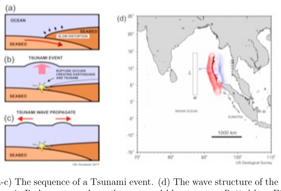Figure 1: (a-c) The sequence of a Tsunami event. (d) The wave structure of the 2004 Indian Ocean Tsunami. Red wave travels to the west and blue to east. Dotted box: Effective area $L\times W$ for the initial tsunami wave generated along the fault line (See Question 1).

Part 1. Energy of tsunami

The ocean floor seismic rupture suddenly displaces a large body of water above it along the fault line as shown in Figure 1. This excess body of water will be dissipated as tsunami waves that mainly propagate to the left and right. Let us make a simple model of the excess body of water with triangular cross section as shown in Figure 2. The initial water displacement is $h=5\text{m}$ covering a large area of fault line of $L=1400\text{km}$ and width $W=150\text{km}$. (Note that $h$ is really in meter, very small compared to $L$ and $W$).

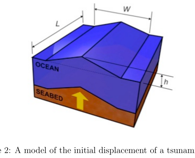Figure 2: A model of the initial displacement of a tsunami wave.

1.A. Calculate the excess energy that will be dissipated as tsunami! Assume that this excess body of water is at rest right after the seismic event.

1.B. Compare this energy with the Hiroshima atomic bomb that equals to 12500 tons of TNT explosion. One ton of TNT explosion yields $4.2\times 10^9\text{J}$ of energy.

Part 2. Speed of tsunami

Tsunami wave, in the open ocean, has small amplitude ($a\sim 5\text{m}$), extremely long wavelength ($\lambda \sim 100\text{km}$) and travels on a very deep ocean ($d\sim 5\text{km}$). Thus, surprisingly, tsunami can be considered as “shallow water waves” where $a\ll d\ll \lambda$. Here the speed of tsunami (or phase velocity) is given as: v = \sqrt{gd} \tag{1}

Let us make a very simple derivation of the tsunami speed by using a simple model of one half tsunami wave using a water tank model as shown below. The water is tilting back and forth from left to right given a slight initial imbalance of height. Thus the height $a$ will oscillate with time. Let us assume that the width of the water tank is half the wavelength of the tsunami wave $\lambda$. The length of water tank is $L$. Note: For tsunami (shallow water) wave, we assume: $a\ll d\ll \lambda$.

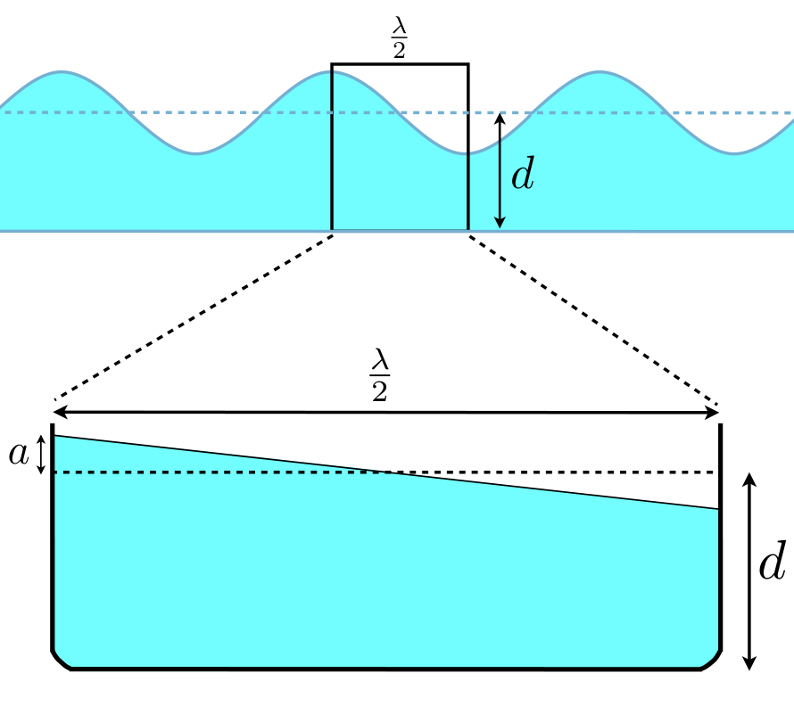Figure 3: Water tank model of a tsunami wave to estimate its wave velocity.

2.A. Write down the horizontal velocity of the water element as a function of horizontal position $x$, $a$ and/or its derivative. Hint: the velocity at the edge of the water tank is zero.

2.B. Express the total kinetic and potential energy of the system in terms of $a$ and/or its derivative!

2.C. Show that the system exhibits a simple harmonic oscillator. Calculate the period of oscillation $T$ of the water!

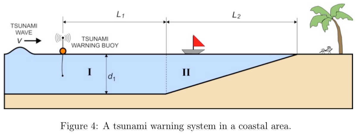Figure 4: A tsunami warning system in a coastal area.

2.D. The tsunami displaces wave with wavelength $\lambda$ in a time period $T$. The wave speed or “phase velocity” is given as: $v=\lambda /T$. Show that: $v\propto \sqrt{gd}$ ($\propto$ means proportional to).

Part 3. Tsunami warning system

Use the tsunami speed equation as given in Eq. 1 above.

3.A. Calculate the average tsunami speed and period in the Indian ocean with depth $d=4000\text{m}$ and a long wavelength of $\lambda =100\text{km}$. What object travels close to that speed? (bike, car, passenger jet plane?).

3.B. A tsunami warning system is installed near a coastal region with the seafloor profile that can be modeled as shown in Figure 4: a constant depth followed by a linearly decreasing depth region. We have a tsunami warning buoy that can detect a tsunami wave front at $t=0$. Calculate the time $\Delta t$ when the tsunami will hit the land!

Part 4. Tsunami characteristics on land impact

In the ocean where the seafloor depth is constant (region I) the tsunami waves has a characteristic height $h$ and coming to the land with linearly increasing ocean floor (region II).

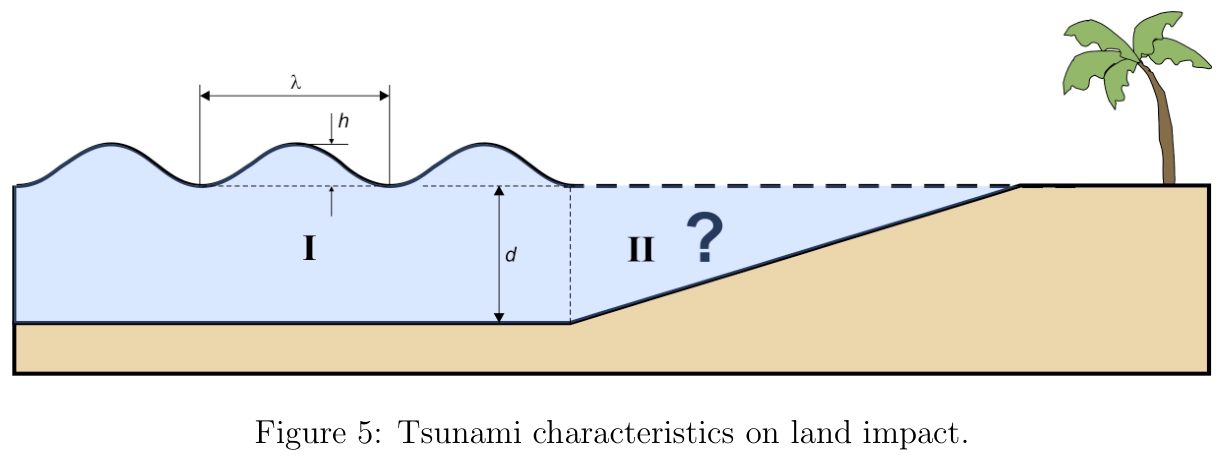Figure 5: Tsunami characteristics on land impact.

4.A. Investigate what happens to the tsunami wave height $h$ as it comes crashing to land. Express the relationship of $h$ as a function of depth $d$. Hint: The period of the tsunami wave is constant everywhere.

4.B. Sketch the tsunami wave as it approaches the land.

4.C. Estimate the height of tsunami wave crashing to Aceh coast (Sumatra, Indonesia) with final depth of $2\text{m}$ (before the wave breaks) coming from Indian ocean with initial wave height of $5\text{m}$ and depth of $4000\text{m}$. Comment on your finding to explain the devastating effect of tsunami.

Part 5. Tsunami Drawback effect

An early warning sign of the incoming tsunami is the “drawback effect” where the sea water near the beach recedes significantly for hundreds of meter and for about half the tsunami period (about few minutes). An observer may be attracted to the exposed beach unaware of the oncoming danger. (In the 2004 Indian Ocean Tsunami event a little tourist boy in Thailand saved the lives of many because he learnt about this effect from school.)

Let us explore this drawback effect by the following model. Assume that we put a test buoy $B$ on the water surface that will track the water particle there. Note that there are two movements: First is the cyclic up and down movement with a period $T=v_0/\lambda$ where $v_0$ is the phase velocity of the wave, and second: the horizontal movement because the buoy is dragged by the traveling wave, but with the speed less than the wave phase velocity $v_0$. Thus to track the trajectory of buoy $B$ we can use a Yo-Yo model which rotates with period $T$ but the center moves with speed less than $v_0$.

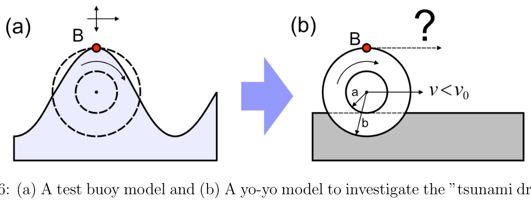Figure 6: (a) A test buoy model and (b) A yo-yo model to investigate the “tsunami drawback effect”.

5.A. Sketch the trajectory of the buoy $B$ as a function of distance as the “Yo-Yo” rolls.

5.B. Highlight your observation that explains the tsunami “drawback” effect!

Fonte: Testo (PDF) — p.1 Topic: Fluid Mechanics, Oscillations & Waves Metodi: Energy Conservation Method, Simple Harmonic Motion Analysis, Dimensional Analysis, Physical Modeling Competenze: Physical Reasoning, Estimation & Approximation, Mathematical Modeling Objects: Container

Tsunami Data limite 31 maggio 2012

**Constanti: **

• Accelerazione gravitazionale: $g=9.8{\text{m/s}}^2$
• densità dell’acqua: $\rho =1000{\text{kg/m}}^3$

Il tsunami è un enorme fenomeno di onde oceaniche generato da un improvviso spostamento dell’acqua a causa dell’attività sismica oceanica (terremoto). Lo tsunami è estremamente devastante per la popolazione umana che vive nella regione costiera. Gli esempi recenti sono lo tsunami dell’Oceano Indiano (2004) e lo tsunami del Tohoku-Giappone (2011) che hanno richiesto rispettivamente 230.000 e 15.000 vite.

In questo problema esploreremo le basi fisiche del tsunami che ci aiuteranno a comprendere alcune delle sue caratteristiche fondamentali e a diffondere alcune conoscenze che potrebbero salvare vite in caso di catastrofe. In questo problema useremo alcuni dati stimati del tsunami dell’Oceano Indiano del 2004 prodotto da un terremoto al largo della costa di Sumatra, in Indonesia come mostrato di seguito.

**Figura 1: ** (a-c) La sequenza di un evento tsunami. d) La struttura delle onde del tsunami dell’Oceano Indiano del 2004. L’onda rossa viaggia verso ovest e l’onda blu verso est. Cassa puntata: area effettiva $L\times W$ per l’onda iniziale di tsunami generata lungo la linea di rottura (vedi domanda 1).

Parte 1. Energia dello tsunami

La rottura sismica del fondo oceanico sposta improvvisamente un grande corpo d’acqua sopra di esso lungo la linea di rottura come mostrato nella Figura 1. Questo eccesso di acqua si disperderà come onde di tsunami che si propagano principalmente a sinistra e a destra. Fate un modello semplice del corpo d’acqua in eccesso con sezione trasversale triangolare come mostrato alla Figura 2. Il spostamento iniziale dell’acqua è $h=5\text{m}$ che copre una grande area di linea di rottura di $L=1400\text{km}$ e larghezza $W=150\text{km}$. (Ricorda che $h$ è realmente in metro, molto piccolo rispetto a $L$ e $W$).

**Figura 2: ** Un modello del spostamento iniziale di un’onda di tsunami.

1.A. Calculate the excess energy that will be dissipated as tsunami! Supponiamo che questo eccesso di acqua sia in riposo subito dopo l’evento sismico.

1.B. Compare this energy with the Hiroshima atomic bomb that equals to 12500 tons of TNT explosion. Una tonnellata di esplosione di TNT produce $4.2\times 10^9\text{J}$ di energia.

Parte 2. Velocità dello tsunami

L’onda tsunami, nell’oceano aperto, ha una piccola amplitudine ($a\sim 5\text{m}$), lunghezza d’onda estremamente lunga ($\lambda \sim 100\text{km}$) e viaggia su un oceano molto profondo ($d\sim 5\text{km}$). Pertanto, sorprendentemente, i tsunami possono essere considerati “onde di acqua poco profonda” dove $a\ll d\ll \lambda$. Qui la velocità dello tsunami (o velocità di fase) è data come: v = \sqrt{gd} \tag{1}

Facciamo una derivazione molto semplice della velocità del tsunami utilizzando un modello semplice di una metà di onda di tsunami utilizzando un modello di serbatoio d’acqua come mostrato di seguito. L’acqua si tende avanti e indietro da sinistra a destra, dato un lieve squilibrio iniziale di altezza. In questo modo l’altezza $a$ oscilla nel tempo. Let us assume that the width of the water tank is half the wavelength of the tsunami wave $\lambda$. La lunghezza del serbatoio d’acqua è $L$. Nota: per l’onda di tsunami (acqua bassa) supponiamo: $a\ll d\ll \lambda$.

**Figura 3: ** Modello di serbatoio d’acqua di un’onda di tsunami per stimare la sua velocità d’onda.

2.A. Scrivere la velocità orizzontale dell’elemento acqua come funzione della posizione orizzontale $x$, $a$ e/o della sua derivata. Suggerimento: la velocità al bordo del serbatoio d’acqua è zero.

2.B. Esprimere l’energia cinetica e potenziale totale del sistema in termini di $a$ e/o derivata!

2.C. Mostri che il sistema presenta un semplice oscillatore armonico. Calcolare il periodo di oscillazione $T$ dell’acqua!

**Figura 4: ** Un sistema di allarme tsunami in una zona costiera.

2.D. Lo tsunami spostano l’onda con lunghezza d’onda $\lambda$ in un periodo di tempo $T$. La velocità d’onda o “velocità di fase” è data come: $v=\lambda /T$. Indicare che: $v\propto \sqrt{gd}$ ($\propto$ significa proporzionale a).

Parte 3. Sistema di avvertimento tsunami

Utilizzare l’equazione di velocità del tsunami come indicato in Eq. Uno sopra.

3.A. Calcolare la velocità e il periodo medio dello tsunami nell’oceano indiano con profondità $d=4000\text{m}$ e lunghezza d’onda $\lambda =100\text{km}$. Quale oggetto si sta muovendo vicino a questa velocità? (bicicletta, auto, aereo aerei passeggeri?).

3.B. Viene installato un sistema di allarme per tsunami vicino a una regione costiera con un profilo del fondo marino che può essere modellato come mostrato alla figura 4: una profondità costante seguita da una regione di profondità che diminuisce linearmente. Abbiamo una boia di avvertimento per i tsunami che può rilevare un’onda di tsunami a $t=0$. Calculate the time $\Delta t$ when the tsunami will hit the land!

Parte 4. Caratteristiche dei tsunami sull’impatto sulla terra

Nell’oceano dove la profondità del fondo marino è costante (regione I) le onde di tsunami hanno un’altezza caratteristica $h$ e arrivano sulla terra con un aumento lineare del fondo oceanico (regione II).

**Figura 5: ** Caratteristiche dei tsunami sull’impatto sul suolo.

4.A. Investigare cosa accade all’altezza delle onde di tsunami $h$ quando si schianta a terra. Esprimere la relazione di $h$ come funzione di profondità $d$. L’epoca dell’onda tsunami è costante ovunque.

4.B. Segna l’onda di tsunami mentre si avvicina alla terraferma.

4.C. Estimare l’altezza dell’onda di tsunami che si schianta verso la costa di Aceh (Sumatra, Indonesia) con una profondità finale di $2\text{m}$ (prima delle pause d’onda) provenienti dall’oceano indiano con un’altezza di onda iniziale di $5\text{m}$ e una profondità di $4000\text{m}$. Commenta le sue scoperte per spiegare l’effetto devastante dello tsunami.

Parte 5. Effetto di riduzione dei tsunami

Un segno di avvertimento precoce del tsunami in arrivo è l‘“effetto di ritiro” quando l’acqua del mare vicino alla spiaggia si allontana significativamente per centinaia di metri e per circa la metà del periodo di tsunami (circa pochi minuti). Un osservatore può essere attratto dalla spiaggia esposta senza essere consapevole del pericolo imminente. (Nel tsunami dell’Oceano Indiano del 2004 un ragazzino turistico in Thailandia salvò la vita di molti perché apprese di questo effetto a scuola.)

Esploriamo questo effetto svantaggio con il modello seguente. Supponiamo di mettere una boia di prova $B$ sulla superficie dell’acqua che traccia la particella d’acqua lì. Si noti che ci sono due movimenti: primo è il movimento ciclico su e giù con un periodo $T=v_0/\lambda$ dove $v_0$ è la velocità di fase dell’onda, e secondo: il movimento orizzontale perché la boia è trascinata dall’onda in movimento, ma con la velocità inferiore alla velocità di fase dell’onda $v_0$. Per quindi tracciare la traiettoria della boia $B$ possiamo utilizzare un modello Yo-Yo che ruota con periodo $T$ ma il centro si muove a velocità inferiore a $v_0$.

**Figura 6: ** (a) Modello di boia di prova e (b) Modello di yo-yo per indagare sull‘“effetto di avversità dei tsunami”.

5.A. Segnare la traiettoria della boia $B$ in funzione della distanza in cui i rulli “Yo-Yo” ruotano.

5.B. Fate notare la vostra osservazione che spiega l’effetto “retro” dello tsunami!

Fonte: Testo (PDF) — p.1 Topic: Fluid Mechanics, Oscillations & Waves Metodi: Energy Conservation Method, Simple Harmonic Motion Analysis, Dimensional Analysis, Physical Modeling Competenze: Physical Reasoning, Estimation & Approximation, Mathematical Modeling Objects: Container

Falling Ball Magnet — Deadline June 30, 2012

A solid ball magnet (with uniform permanent magnetization $M_0$) of mass $m$ and radius $a$ is dropped from the top of a metallic conducting tube (whose inner radius is a tiny bit larger than $a$ and has thickness $\Delta \ll a$). Denote the conductivity of the metal by $\sigma$ and the gravitational acceleration by $g$. As the ball magnet is released from rest, it will start falling and eventually it will reach a certain terminal velocity. Some details can be found in the schematics below, and several simplifying assumptions are as follows:

• Ignore air friction as well as friction between the ball and the tube.
• For simplicity, one may assume that the magnetization of the ball is oriented vertically down and the ball does not rotate as it falls down.

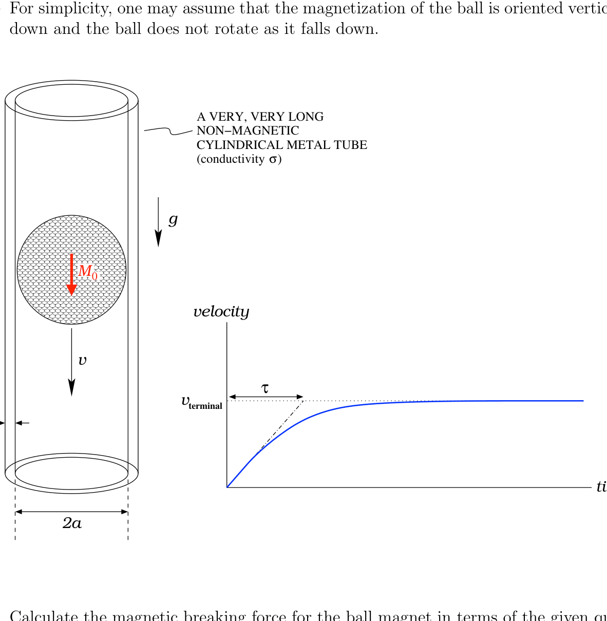
(a). Calculate the magnetic breaking force for the ball magnet in terms of the given quantities and relevant physical constants.

(b). Calculate the terminal velocity of the magnetic ball.

(c). Calculate the time scale $\tau$ for the magnetic ball to reach terminal velocity in terms of the given quantities and relevant physical constants.

Fonte: Testo (PDF) — p.1 Topic: Electromagnetic Induction, Magnetism Metodi: Faraday’s Law of Induction, Lenz’s Law, Free-Body Diagram, Differential Equations Competenze: Physical Reasoning, Mathematical Modeling Objects: Magnet, Tube, Ball

Magnetto a palla cadente Data limite 30 giugno 2012

Un magnete a sfera solida (con una magnetizzazione permanente uniforme $M_0$) di massa $m$ e raggio $a$ viene scaricato dalla parte superiore di un tubo conduttore metallico (il cui raggio interno è leggermente più grande di $a$ e ha spessore $\Delta \ll a$). Nota la conducibilità del metallo con $\sigma$ e l’accelerazione gravitazionale con $g$. Quando il magnete della palla viene rilasciato dal riposo, inizierà a cadere e alla fine raggiungerà una certa velocità terminale. Alcuni dettagli sono riportati nei schemi di seguito, e alcune ipotesi semplificanti sono le seguenti:

• Ignora l’attrito dell’aria e l’attrito tra la palla e il tubo.
• Per semplicità, si può supporre che la magnetizzazione della palla sia orientata verticalmente verso il basso e la palla non ruota mentre cade.

(a). Calcolare la forza di rottura magnetica del magnete a sfera in termini di quantità e di costanti fisiche rilevanti.

(b). Calcolare la velocità terminale della palla magnetica.

(c). Calcolare la scala temporale $\tau$ per la palla magnetica per raggiungere la velocità terminale in termini di quantità e di costanti fisiche rilevanti.

Fonte: Testo (PDF) — p.1 Topic: Electromagnetic Induction, Magnetism Metodi: Faraday’s Law of Induction, Lenz’s Law, Free-Body Diagram, Differential Equations Competenze: Physical Reasoning, Mathematical Modeling Objects: Magnet, Tube, Ball

Relativistic Images — Deadline June 30, 2012

As the old proverb goes, “seeing is believing”, and since seeing depends on light, what we see is highly dependent on the nature of light. These following problems aim to investigate the peculiarities of vision in the light of Relativity theory, particularly those arising from the effect of light’s nonzero travel time.

Part 1. Cameras

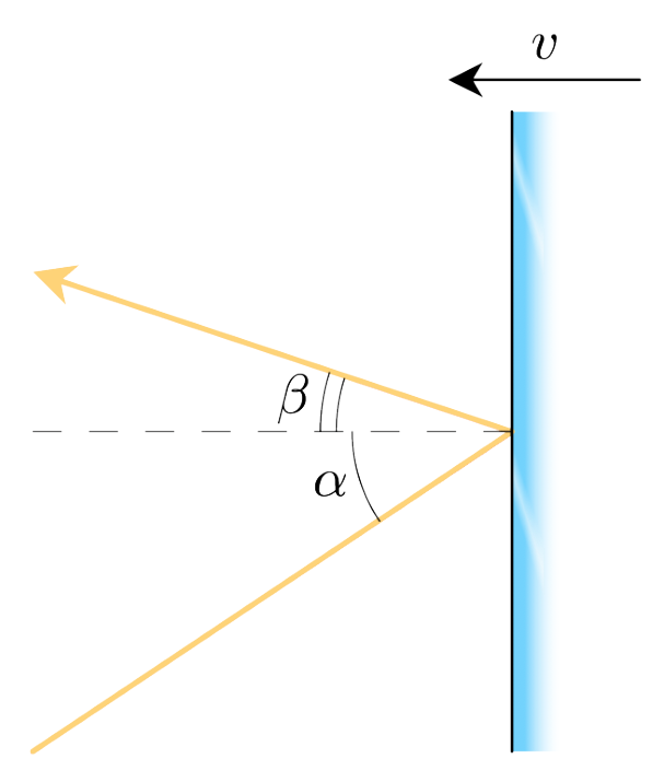
1.A. A perfectly reflecting mirror moves at a relativistic speed $v$ in a direction normal to the plane of its surface. At a certain moment, a narrow beam of light strikes the mirror at an angle of incidence $\alpha$. Determine the angle of reflection $\beta$ of the beam, and show that in the limit of small angles, the ratio of $\alpha$ and $\beta$ is given by \frac{\alpha}{\beta} = \frac{c+v}{c-v} \tag{1}

1.B. Consider a simplified view of image formation in a camera, wherein said device works by capturing light from an object and projecting it onto a screen. If the object is far away, light from it would obviously be focused at the focal point of the camera’s lens.

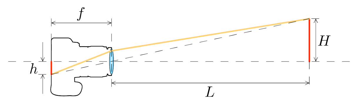
It is easily shown that the size of the image formed on the screen of the camera, for an object of size $H$ at a distance $L$ from the camera, is given by $h=Hf/L$.

Suppose now that the camera is approaching the object at a relativistic speed $v$ while rapidly taking a photograph; assume the distance between the camera and the object is still $L$.

• (a) How will the image on the moving camera screen look (bigger or smaller) compared to the original case where the camera is at rest?
• (b) At what rate will the height of the image on the screen be changing at this instant?

1.C. A camera with video-recording capability, width $D$, lens focal length $f$ and a clock attached in front of it is moving relativistically with speed $v$ towards a perfectly reflecting plane mirror as shown in the figure below.

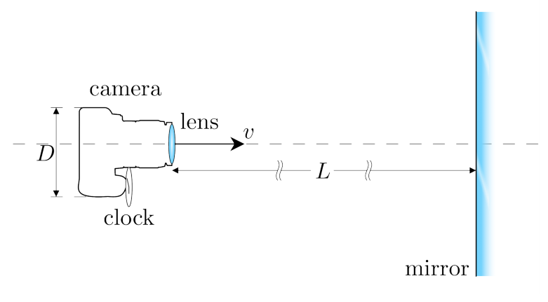
• (a) At a certain moment, the camera is located at a distance $L$ from the mirror in the mirror’s rest frame. Determine the rate of change of the camera image’s width as recorded by the camera itself, given that $L\gg d$.
• (b) At that time an observer moving together with the camera notes that the difference between the reading of the camera’s clock and the image’s clock is $A$ seconds and that the ticking speed of one clock is $B$ times faster than the other. Using this information, find the distance between the camera and the mirror as seen in the rest frame of the mirror, given that $A>0$ and $B>1$.
• (c) Show that at the moment the camera reaches the mirror, both its clock and its image’s will show the same time.

Part 2. Expanding Stars

A perfectly spherical star of spectral class G initially has a radius $R_0$. All of a sudden, a cataclysmic event at $t=0$ in the star’s rest frame causes it to start expanding at a constant relativistic rate $dR/dt=v$. An observer on Earth, at a distance $L\gg R$ from the star, is observing this strange phenomenon. The Earth frame can be treated as an inertial frame.

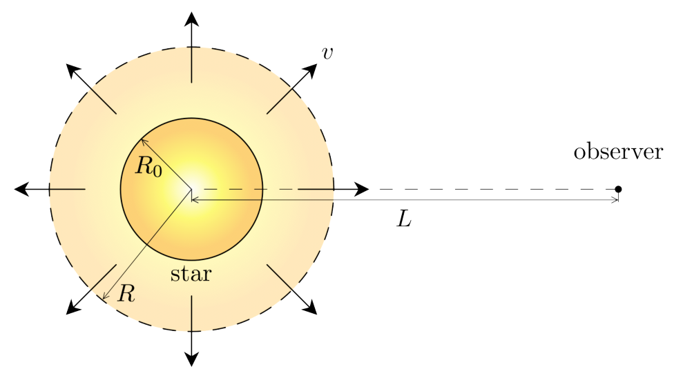
2.A. Determine the apparent angular size of the star as a function of time, $\theta (t)$, as seen by the observer. Hint: it may be a good idea to plot this function.

2.B. When the star reaches a certain radius $R_m$, its light suddenly dies out. Describe, both qualitatively and quantitatively, the shape of the star as seen by the observer, from the moment the star’s radius reaches $R_m$, and onwards to eternity.

Assume the star is a perfect blackbody so that light from the star’s interior cannot reach the observer on Earth.

Fonte: Testo (PDF) — p.1 Topic: Special Relativity, Geometric Optics Metodi: Lorentz Transformation, Thin Lens & Mirror Equation, Ray Tracing, Physical Modeling Competenze: Physical Reasoning, Mathematical Modeling Objects: Mirror, Lens, Star

Image relative Data limite 30 giugno 2012

Come dice il vecchio proverbio, “vedere è credere”, e poiché vedere dipende dalla luce, ciò che vediamo dipende fortemente dalla natura della luce. Questi seguenti problemi mirano ad indagare sulle peculiarità della visione alla luce della teoria della relatività, in particolare quelle derivanti dall’effetto del tempo di viaggio non zero della luce.

Parte 1. Cammere

1.A. Uno specchio perfettamente riflesso si muove a velocità relativistica $v$ in una direzione normale al piano della sua superficie. In un certo momento, un raggio di luce stretta colpisce lo specchio ad un angolo di incidenza $\alpha$. Determinare l’angolo di riflessione $\beta$ del fascio e mostrare che nel limite di angoli piccoli, il rapporto tra $\alpha$ e $\beta$ è dato da \frac{\alpha}{\beta} = \frac{c+v}{c-v} \tag{1}

1.B. Considerate una visualizzazione semplificata della formazione di immagini in una fotocamera, in cui tale dispositivo funziona catturando la luce da un oggetto e proiettandola su uno schermo. Se l’oggetto è lontano, la luce da esso si focalizzerà ovviamente al punto focale dell’obiettivo della fotocamera.

Si può facilmente dimostrare che la dimensione dell’immagine formata sullo schermo della fotocamera, per un oggetto di dimensioni $H$ a distanza $L$ dalla fotocamera, è data da $h=Hf/L$.

Supponiamo ora che la fotocamera si avvicini all’oggetto a una velocità relativistica $v$ mentre prende rapidamente una fotografia; supponiamo che la distanza tra la fotocamera e l’oggetto sia ancora $L$.

• a) Come sarà l’immagine sullo schermo della fotocamera in movimento (più grande o più piccolo) rispetto al caso originale in cui la fotocamera è in riposo?
• (b) A che velocità cambierà l’altezza dell’immagine sullo schermo in questo istante?

Una fotocamera con capacità di registrazione video, larghezza $D$, lunghezza focale $f$ e un orologio fissato davanti si muove relativisticamente con velocità $v$ verso uno specchio piano perfettamente riflesso come mostrato nella figura seguente.

• a) In un certo momento, la telecamera si trova a una distanza $L$ dallo specchio nel quadro di riposo dello specchio. Determinare il tasso di variazione della larghezza dell’immagine della fotocamera, come registrato dalla fotocamera stessa, data la $L\gg d$.
• (b) In quel momento un osservatore che si muove insieme alla macchina fotografica osserva che la differenza tra la lettura dell’orologio della macchina fotografica e l’orologio dell’immagine è di $A$ secondi e che la velocità di ticchatura di un orologio è $B$ volte più veloce dell’altro. Con queste informazioni, si trova la distanza tra la fotocamera e lo specchio come si vede nella cornice del resto dello specchio, dato che $A>0$ e $B>1$.
• (c) Mostra che nel momento in cui la fotocamera raggiunge lo specchio, sia il suo orologio che l’immagine mostreranno lo stesso orario.

Parte 2. Le stelle in espansione

Una stella perfettamente sferica di classe spettrale G ha inizialmente un raggio $R_0$. All’improvviso, un evento cataclismico a $t=0$ nel quadro di riposo della stella fa sì che inizi a espandersi a un ritmo relativistico costante $dR/dt=v$. Un osservatore sulla Terra, a una distanza $L\gg R$ dalla stella, sta osservando questo strano fenomeno. Il telaio terrestre può essere trattato come un telaio inerziale.

2.A. Determinare la dimensione angolare apparente della stella in funzione del tempo, $\theta (t)$, come osservato dall’osservatore. Suggerimento: potrebbe essere una buona idea tracciare questa funzione.

Quando la stella raggiunge un certo raggio di $R_m$, la sua luce si spegne improvvisamente. Descrivere, qualitativamente e quantitativamente, la forma della stella osservata dall’osservatore, dal momento in cui il raggio raggiunge $R_m$, e in avanti fino all’eternità.

Supponiamo che la stella sia un corpo nero perfetto, in modo che la luce dall’interno della stella non possa raggiungere l’osservatore sulla Terra.

Fonte: Testo (PDF) — p.1 Topic: Special Relativity, Geometric Optics Metodi: Lorentz Transformation, Thin Lens & Mirror Equation, Ray Tracing, Physical Modeling Competenze: Physical Reasoning, Mathematical Modeling Objects: Mirror, Lens, Star

Pouring Water into a Tube — Deadline July 31, 2012

Part 1.

A steady stream of water from a pipe valve slowly fills up a relatively slender cylindrical tube of height $l_0=1\text{m}$ and base area $A=1.26\times 10^{-3}{\text{m}}^2$. As the tube is being filled up with water, a microphone records the sound that is being produced. The spectrogram of the recorded sound signal reveals the time evolution of the prominent audible frequencies as the water level in the tube rises. The details are illustrated in the following schematics:

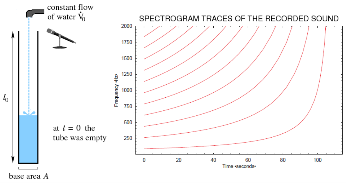
Based on the available information of the setup and the data given, determine reasonably reliable numerical estimates for the following quantities:

1.A. the sound speed $c_s$ under local atmospheric conditions (unit: m/s)

1.B. the flow rate of the water stream ${\dot{V}}_0$ into the tube (unit: m³/s)

For the purpose of aiding analysis and calculations, a larger version of the above spectrogram plot is provided below (page 4 of the original exam paper).

Part 2.

On another occasion, a similar experiment is performed under slightly different conditions and settings. A steady stream of water slowly fills up a relatively slender cylindrical tube of height $l_0=1\text{m}$ and base area $A=1.26\times 10^{-3}{\text{m}}^2$, but this time the side of the tube has a small hole at a certain location. Again, a microphone records the sound that is being produced as the tube is being filled up with water. The gravitational acceleration is $g=9.8{\text{m/s}}^2$. The settings and the resulting spectrogram traces are shown in the schematics below:

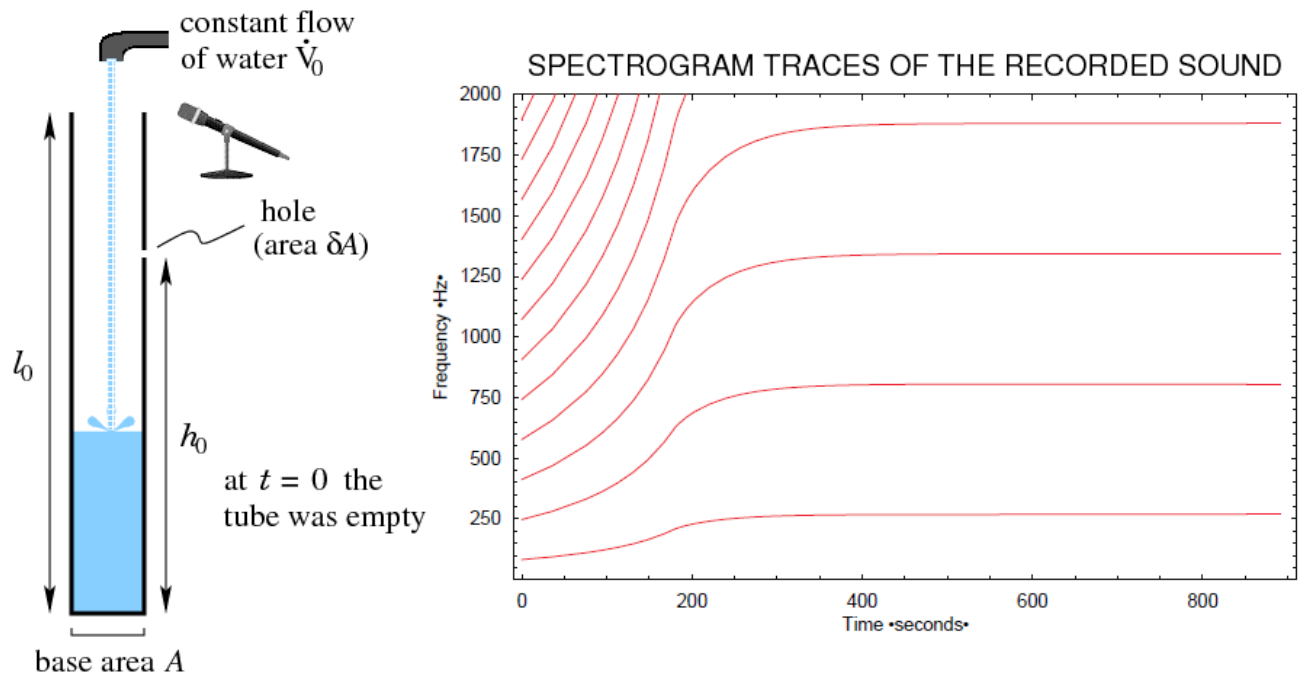
Based on the available information of the setup and the data given, determine reasonably reliable numerical estimates for the following quantities:

2.A. the sound speed $c_s$ under local atmospheric conditions (unit: m/s)

2.B. the flow rate of the water stream ${\dot{V}}_0$ into the tube (unit: m³/s)

2.C. the height $h_0$ where the hole is located (unit: m)

2.D. the area $\delta A$ of the hole (unit: m²)

Note: Ignore the effect of vena contracta (i.e. diameter contraction) in the jet of water leaking from the hole when the water level is above the hole position.

Larger spectrogram plots

Spectrogram Plot for Part I:

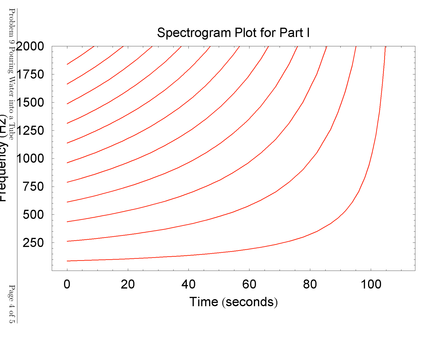
Spectrogram Plot for Part II:

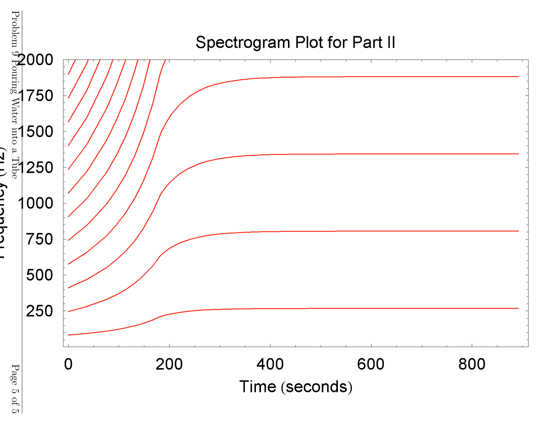
Fonte: Testo (PDF) — p.1 Topic: Oscillations & Waves, Fluid Mechanics Metodi: Wave Equation, Bernoulli’s Equation, Experimental Data Analysis, Continuity Equation Competenze: Experimental Data Analysis, Estimation & Approximation, Physical Reasoning Objects: Tube

Rivogare acqua in un tubo Scadenza 31 luglio 2012

Parte 1.

Un flusso costante di acqua proveniente da una valvola di tubo riempie lentamente un tubo cilindrico relativamente sottile di altezza $l_0=1\text{m}$ e di superficie di base $A=1.26\times 10^{-3}{\text{m}}^2$. Mentre il tubo si riempie di acqua, un microfono registra il suono che viene prodotto. Lo spettrogramma del segnale sonoro registrato rivela l’evoluzione temporale delle frequenze audibili più importanti man mano che il livello dell’acqua nel tubo sale. I dettagli sono illustrati nei seguenti schemi:

Sulla base delle informazioni disponibili sull’impianto e dei dati forniti, determinare stime numeriche ragionevolmente affidabili per le seguenti quantità:

1.A. la velocità sonora $c_s$ in condizioni atmosferiche locali (unità: m/s)

1.B. il flusso di corrente d’acqua ${\dot{V}}_0$ nel tubo (unità: m3/s)

Ai fini dell’analisi e dei calcoli, una versione più ampia del diagramma di spettrogramma di cui sopra è riportata di seguito (pagina 4 del documento di esame originale).

Parte 2.

In un’altra occasione, un esperimento simile viene eseguito in condizioni e impostazioni leggermente diverse. Un flusso di acqua costante riempie lentamente un tubo cilindrico relativamente sottile di altezza $l_0=1\text{m}$ e di superficie di base $A=1.26\times 10^{-3}{\text{m}}^2$, ma questa volta il lato del tubo ha un piccolo buco in una certa posizione. Ancora una volta, un microfono registra il suono che viene prodotto mentre il tubo viene riempito di acqua. L’accelerazione gravitazionale è $g=9.8{\text{m/s}}^2$. Le impostazioni e le tracce dello spettroogramma risultanti sono riportate nelle schemiche di seguito:

Sulla base delle informazioni disponibili sull’impianto e dei dati forniti, determinare stime numeriche ragionevolmente affidabili per le seguenti quantità:

2.A. la velocità sonora $c_s$ in condizioni atmosferiche locali (unità: m/s)

2.B. il flusso di corrente d’acqua ${\dot{V}}_0$ nel tubo (unità: m3/s)

2.C. l’altezza $h_0$ in cui si trova il buco (unità: m)

2.D. la superficie $\delta A$ del buco (unità: m2)

Nota: Ignorare l’ effetto della vena contracta (cioè diametro di contrazione) nel getto di acqua che scorre dal buco quando il livello dell’acqua è superiore alla posizione del buco.

# Piu’ grandi grafici di spettrogrammi

Spettro di spettro per la parte I:

Spettro di spettro della parte II:

Fonte: Testo (PDF) — p.1 Topic: Oscillations & Waves, Fluid Mechanics Metodi: Wave Equation, Bernoulli’s Equation, Experimental Data Analysis, Continuity Equation Competenze: Experimental Data Analysis, Estimation & Approximation, Physical Reasoning Objects: Tube

Tides — Deadline July 31, 2012

The Moon’s gravitational pull is commonly known to be among the main reasons for cyclic sea level changes, or tides. In this problem, you are asked to determine a shape of the ocean water surface and a tide height. To estimate the influence of the Moon, it will suffice to consider the simplest model of an Earth-Moon system (part 1). A detailed and correct description is to be based on a more sophisticated model (part 2).

The only objects considered in the problem are Earth and Moon. The influence of the Sun and the rest of planets in the solar system will be neglected (except for question 2.G where the Earth-Sun system is considered). Assume also that the Earth surface is completely covered by water and the ocean floor doesn’t prevent the water movement. You should solve the problem in terms of gravitational potential.

Potential of the gravitational field is the ratio between the potential energy of a material point placed into the gravitational field and the mass of the point. It is analogous to the electric potential. The gravitational potential of the point mass $m$ at a distance $r$ from it is: \varphi = -\frac{Gm}{r} + \text{const} \tag{1} where $G=6.67\times 10^{-11}{\text{N⋅m}}^2/{\text{s}}^2$ gravitational constant.

The arbitrary constant is governed by conditions of the potential normalization. The value of the constant does not matter, so while solving the problem, one can drop all the constants from expressions for the gravitational potential.

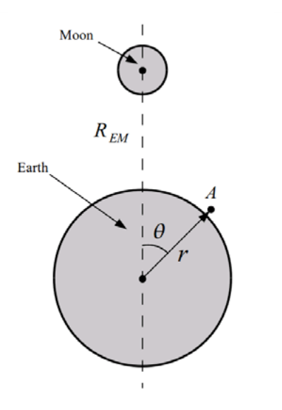Figure 1: Earth and Moon.

Earth-Moon system parameters:

• Earth Mass: $M_E=6.0\times 10^{24}\text{kg}$
• Moon Mass: $M_M=7.4\times 10^{22}\text{kg}$
• Earth Radius: $R_E=6.4\times 10^6\text{m}$
• Earth-Moon distance: $R_{EM}=3.8\times 10^8\text{m}$

Part 1. Simplest model

In the simplest model, the revolution of Earth and Moon about the barycentre and their rotation around axes are neglected. Assume that Moon and Earth are fixed and the distance between their centers is $R_{EM}$ (fig. 1).

1.A. Write down the expressions for gravitational potentials ${\phi }_E(r)$ and ${\phi }_M(r,\theta )$ of the field created by Earth and Moon respectively in a point $A$ located close to the Earth surface at a distance $r$ from its centre and at an angle $\theta$ to the Earth-Moon line (fig. 1).

1.B. Using the approximation $(1+x{)}^{\alpha }\approx 1+\alpha x$, write down the expression for the resultant potential: $\phi (r,\theta )={\phi }_E(r)+{\phi }_M(r,\theta )$. Discard all constants.

1.C. The ocean water surface is equipotential. Which points at the Earth surface correspond to minimum and maximum water levels? Sketch a water surface shape, indicate the Moon location on your sketch.

1.D. The tidal height is a half of the difference between maximal and minimal marks of the water level. Calculate the value of the tidal height.

Part 2. More sophisticated and correct model

In this part you should take account of the Earth and Moon orbiting around their barycentre. Neglect as before the rotation of the Earth about its axis.

2.A. Assuming that Earth and Moon move in circular orbits, find the distance $d$ between the centre of Earth and the Earth-Moon system barycentre. Find the angular velocity $\omega$ of the system rotation. Express $d$ and $\omega$ in terms of the Earth-Moon system parameters.

2.B. There is centrifugal force in the rotating frame of reference. This force can be taken into account by introducing a centrifugal potential ${\phi }_C$. Express the centrifugal potential in terms of both the distance $x$ to the axis of rotation and the angular velocity $\omega$.

2.C. Write down the expression for the centrifugal potential ${\phi }_C(r,\theta )$ in the point $A$ (fig. 1). As before, discard all the constants.

2.D. Write down the expression for the total potential, $\phi (r,\theta )={\phi }_E(r)+{\phi }_M(r,\theta )+{\phi }_C(r,\theta )$. When writing ${\phi }_M(r,\theta )$, use the approximation $(1+x{)}^{\alpha }\approx 1+\alpha x+\frac{\alpha (\alpha -1)}{2}{x}^2$ to retain the dependence on angle $\theta$.

2.E. Which points at the Earth surface correspond to minimum and maximum water levels? Sketch a water surface shape; indicate the Moon location on your sketch.

2.F. Calculate the value of the tidal height.

2.G. Consider the Earth-Sun two-body system. Calculate the value of the tidal height caused by the Sun. The Sun mass: $M_s=2.0\times 10^{30}\text{kg}$. The distance between the Earth and the Sun: $R_{ES}=1.5\times 10^{11}\text{m}$.

Fonte: Testo (PDF) — p.1 Topic: Gravitation, Newtonian Mechanics Metodi: Newton’s Law of Gravitation, Approximation & Series Expansion, Symmetry Argument, Physical Modeling Competenze: Physical Reasoning, Mathematical Modeling Objects: Planet, Satellite, Star

Tides Termine del 31 luglio 2012

La forza gravitazionale della Luna è comunemente nota per essere tra le principali ragioni per i cambiamenti ciclici del livello del mare, o maree. In questo problema, si chiede di determinare una forma della superficie dell’acqua oceanica e un’altezza delle maree. Per stimare l’influenza della Luna, basta considerare il modello più semplice di un sistema Terra-Luna (parte 1). Una descrizione dettagliata e corretta deve basarsi su un modello più sofisticato (parte 2).

Gli unici oggetti considerati nel problema sono la Terra e la Luna. L’influenza del Sole e del resto dei pianeti del sistema solare sarà trascurata (ad eccezione della domanda 2.G, in cui viene considerato il sistema Terra-Sol). Supponiamo anche che la superficie terrestre sia completamente coperta da acqua e il fondo oceanico non impedisca il movimento dell’acqua. Dovresti risolvere il problema in termini di potenziale gravitazionale.

Il potenziale del campo gravitazionale è il rapporto tra l’energia potenziale di un punto materiale inserito nel campo gravitazionale e la massa del punto. È analogo al potenziale elettrico. Il potenziale gravitazionale della massa puntaria $m$ a distanza $r$ da essa è: \varphi = -\frac{Gm}{r} + \text{const} \tag{1} dove $G=6.67\times 10^{-11}{\text{N⋅m}}^2/{\text{s}}^2$ è costante gravitazionale.

La costante arbitraria è governata dalle condizioni della normalizzazione potenziale. Il valore della costante non conta, quindi, mentre si risolve il problema, si possono eliminare tutte le costanti dalle espressioni per il potenziale gravitazionale.

**Figura 1: ** Terra e Luna.

Parametri del sistema Terra-Luna:

• Massa terrestre: $M_E=6.0\times 10^{24}\text{kg}$
• Massa lunare: $M_M=7.4\times 10^{22}\text{kg}$
• Radio terrestre: $R_E=6.4\times 10^6\text{m}$
• Distanza Terra-Luna: $R_{EM}=3.8\times 10^8\text{m}$

Parte 1. Modello più semplice

Nel modello più semplice, la rivoluzione della Terra e della Luna intorno al baricentro e la loro rotazione intorno agli assi sono trascurate. Supponiamo che la Luna e la Terra siano fisse e che la distanza tra i loro centri sia $R_{EM}$ (fig. 1).

1.A. Scrivere le espressioni per i potenziali gravitazionali ${\phi }_E(r)$ e ${\phi }_M(r,\theta )$ del campo creato rispettivamente dalla Terra e dalla Luna in un punto $A$ situato vicino alla superficie terrestre a una distanza $r$ dal suo centro e ad un angolo $\theta$ dalla linea Terra-Luna (fig. 1).

1.B. Usando l’approssimazione $(1+x{)}^{\alpha }\approx 1+\alpha x$, annotare l’espressione per il potenziale risultante: $\phi (r,\theta )={\phi }_E(r)+{\phi }_M(r,\theta )$. Scartate tutte le costanti.

La superficie dell’acqua oceanica è equipotenziale. Quali punti della superficie terrestre corrispondono ai livelli minimi e massimi di acqua? Segna una forma della superficie dell’acqua, indica la posizione della Luna sul tuo disegno.

1.D. L’altezza delle maree è la metà della differenza tra i segni massimi e minimi del livello dell’acqua. Calcola il valore dell’altezza delle maree.

Parte 2. Modello più sofisticato e corretto

In questa parte si dovrebbe tenere conto della Terra e della Luna che orbitano attorno al loro baricentro. Negliziare come prima della rotazione della Terra intorno al suo asse.

2.A. Supponendo che la Terra e la Luna si muovano in orbite circolari, si trova la distanza $d$ tra il centro della Terra e il baricentro del sistema Terra-Luna. Trova la velocità angolare $\omega$ della rotazione del sistema. Esprimere $d$ e $\omega$ in termini di parametri del sistema Terra-Luna.

2.B. Nella cornice di riferimento rotante c’è una forza centrifugata. Questa forza può essere presa in considerazione introducendo un potenziale centrifugo ${\phi }_C$. Esprimere il potenziale centrifugo in termini sia della distanza $x$ all’asse di rotazione che della velocità angolare $\omega$.

2.C. Scrivere l’espressione per il potenziale centrifugo ${\phi }_C(r,\theta )$ nel punto $A$ (fig. 1). Come prima, scaricare tutte le costanti.

2.D. Scrivi l’espressione per il potenziale totale, $\phi (r,\theta )={\phi }_E(r)+{\phi }_M(r,\theta )+{\phi }_C(r,\theta )$. Quando si scrive ${\phi }_M(r,\theta )$, si utilizza l’approssimazione $(1+x{)}^{\alpha }\approx 1+\alpha x+\frac{\alpha (\alpha -1)}{2}{x}^2$ per mantenere la dipendenza dall’angolo $\theta$.

2.E. Quali punti della superficie terrestre corrispondono ai livelli minimi e massimi di acqua? Segna una forma della superficie dell’acqua; indica la posizione della Luna sul tuo disegno.

2.F. Calcolare il valore dell’altezza delle maree.

2.G. Considera il sistema a due corpi Terra-Sol. Calcola il valore dell’altezza delle maree causata dal Sole. La massa solare: $M_s=2.0\times 10^{30}\text{kg}$. Distanza tra la Terra e il Sole: $R_{ES}=1.5\times 10^{11}\text{m}$.

Fonte: Testo (PDF) — p.1 Topic: Gravitation, Newtonian Mechanics Metodi: Newton’s Law of Gravitation, Approximation & Series Expansion, Symmetry Argument, Physical Modeling Competenze: Physical Reasoning, Mathematical Modeling Objects: Planet, Satellite, Star